Download
1 / 73
730 likes | 887 Vues
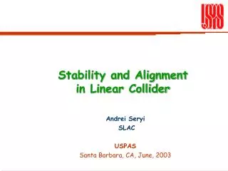
Stability and Alignment in Linear Collider. Andrei Seryi SLAC USPAS Santa Barbara, CA, June, 2003. The Luminosity Challenge. Must jump by a Factor of 10000 in Luminosity !!! (from what is achieved in the only so far linear collider SLC)

E N D
Stability and Alignment in Linear Collider Andrei Seryi SLAC USPAS Santa Barbara, CA, June, 2003
The Luminosity Challenge • Must jump by a Factor of 10000 in Luminosity !!!(from what is achieved in the only so far linear collider SLC) • Many improvements, to ensure this : generation of smaller emittances, their better preservation, … • Including better focusing, dealing with beam-beam, and better stability • Ensure maximal possible focusing of the beams at IP • Optimize IP parameters w.r.to beam-beam effects • Ensure that ground motion and vibrations do not produce intolerable misalignments Lecture 6 Lecture 7 Lecture 8
Stability – tolerance to FD motion IP • Displacement of FD by dY cause displacement of the beam at IP by the same amount • Therefore, stability of FD need to be maintained with a fraction of nanometer accuracy • How would we detect such small offsets of FD or beams? • Using Beam- beam deflection !
Beam-beam deflection Sub nm offsets at IP cause large well detectable offsets (micron scale) of the beam a few meters downstream
What can cause misalignments of FD and other quads? • Initial installation errors • But if static, can eventually correct them out • Non-static effects, such as ground motion (natural or human produced) • In this lecture, we will try to learn how to evaluate effect of ground motion and misalignment on linear collider
What ground motion we are talking about ? • In some languages “Earth” and “ground” called by the same word… • No, we are not talking about Earth orbital motion…
And not so much about earthquakes… World Seismicity: 1975-1995
Ever-present ground motion and vibration and its effect on LC 7sec hum • Fundamental – decrease as 1/w4 • Quiet & noisy sites/conditions • Cultural noise & geology very important • Motion is small at high frequencies… • How small? Cultural noise& geology Power spectral density of absolute position data from different labs 1989 - 2001
Natural ground motion is smallat high frequencies At F>1 Hz the motion can be < 1nm (I.e. much less than beam size in LC) Is it OK? What about low frequency motion? It is much larger… 1 micron 1 nm Rms displacement in different frequency bands. Hiidenvesy cave, Finland
Ground motion in time and space • To find out whether large slow ground motion relevant or not… • One need to compare • Frequency of motion with repetition rate of collider • Spatial wavelength of motion with focusing wavelength of collider Snapshot of a linac Wavelength of misalignment
Two effects of ground motionin Linear Colliders frequency ‘fast motion’ ‘slow motion’ Fc ~ Frep /20 Beam offset due to slow motion can be compensated by feedback May result only in beam emittancegrowth Beam offset cannot be corrected by a pulse-to-pulse feedback operating at the Frep Causes beam offsets at the IP
Focusing wavelengthof a FODO linac FODO linac with beam entering with an offset Betatron wavelength is to be compared with wavelength of misalignment beam quads Focusing wavelength (“betatron wavelength”)
Movie of a Misaligned FODO linacnext page Note the following: Beam follows the linac if misalignment is more smooth than betatron wavelength Resonance if wavelength of misalignment ~ focusing wavelength Spectral response function – how much beam motion due to misalignment with certain wavelength Below, we will try to understand this behavior step by step…
How to predict orbit motion or chromatic dilution Let’s consider a beamline consisting of misaligned quadrupoles with position xi(t)=x(t,si) of the i-th element measured with respect to a reference line. Here si is longitudinal position of the quads. If xabs(t,s) is a coordinate measured in an inertial frame and the reference line passes through the entrance, than x(t,s)= xabs(t,s)- xabs(t,0). We also assume that at t=0 the quads were aligned x(0,s)=0. Misaligned quads. Here xi is quad displacement relative to reference line, and ai is BPM readings. We are interested to find the beam offset at the exit x* or the dispersion hx, produced by misaligned quadrupoles. Let’s assume that bi and di are the first derivatives of the beam offset and beam dispersion at the exit versus displacement of the element i. Then the final offset, measured with respect to the reference line, and dispersion are given by summation over all elements: Is it clear why there is no ai in this formula? Where N is the total number of quads, R and T are 1st and 2nd order matrices of the total beamline, and we also took into account nonzero position and angle of the injected beam at the entrance.
Predicting orbit motion and chromatic dilution … random case Let’s assume now that the beam is injected along the reference line, then: Assume that quads misalignments, averaged over many cases, is zero. Let’s find the nonzero variance Let’s first consider a very simple case. In case of random uncorrelated misalignment we have (sx is rms misalignment, not the beam size) So that, for example And similar for dispersion Now we would like to know what are these b and d coefficients.
Where is the element of transfer matrix from i-th element to the exit Where is the 2nd order transfer matrix from i-th element to the exit Predicting x* and h … what are these bi and di coefficients Let’s consider a thin lens approximation. In this case, transfer matrix of i-th quadrupole is (K>0 for focusing and K<0 for defocusing) A quad displaced by xi produces an angular kick q=Kixiand the resulting offset at the exit will be The coefficient biis therefore The coefficient diis the derivative of di with respect to energy deviation d : Which is equal to
The matrix element from the i-th quad to the exit (N-th quad) is Where is the phase advance from i-th quad and exit. Obviously, Transfer matrices for FODO linac Let’s consider a FODO linac… No, let’s consider, for better symmetry, a (F/2 O D O F/2) linac. Example is shown in the figure on the right side. The quadrupole strength is Ki= K (-1)i+1 (ignoring that first quad is half the length). The position of the quadrupoles is Si= (i –1)L where L is quad spacing. The betatron phase advance m per FODO cell is given by And here bi and bN are beta-functions in the quads. For such regular FODO, the min and max values of beta-functions (achieved in quads) are Since the energy dependence comes mostly from the phase advance (it has large factor of N) and the beta-function variation can be neglected, the second order coefficients are given by
Exercise 5create a FODO linac In this case you will create a fodo linac in MAD for further studies of stability in MatLIAR. The necessary files are in C:\LC_WORK\ex5 The fodo beamline is defined as shown below: LH : DRIF, L = 4.900 ! strength of quads (for 60 degrees per cell) KQ = 1.0 ! length of quad LQ = 0.2/2 QF:QUAD,L=LQ,K1= KQ QD:QUAD,L=LQ,K1=-KQ BPM : MONITOR IP : MONITOR FCELL: LINE=(QF,LH,QD,BPM,QD,LH,QF,BPM) DCELL: LINE=(QD,LH,QF,BPM,QF,LH,QD,BPM) FLCLL:LINE=(2*FCELL) ! You may change the number of cells FODO:LINE=(50*FLCLL,IP) Remember that in MAD K1 is Gradient/Br which is in 1/m2 So, to get the K from the previous page, multiply by quad length Note that initial beta-functions are not specified anywhere in this file. Clever MAD decides that in this case he needs to find a solution where exit and entrance beta-functions are the same (closed solution). When you get the FODO optics, look into fodo_simple.print to get the values for beta and alpha functions at the entrance. You will need to insert these values into the file fodo_init.liar in the Exercise 6.
Exercise 6random misalignments of FODO linac In this case you will use MatLIAR to simulate random misalignments of FODO linac, plot misalignments and orbits, find rms value of orbit motion at the exit, and compare with your analytical predictions. The necessary files are in C:\LC_WORK\ex6 Examples of MatLIAR calls are shown below: Example of misalignments and orbits Make sure to edit the file fodo_init.liar and put correct values of initial beta and alpha functions both in the commands calc_twiss and set_initial
Predicting orbit motion … escaping the complete randomness Now you have everything to calculate b and d coefficients and find, for example, the rms of the orbit motion at the exit for the simplest case – completely random uncorrelated misalignments. Completely random and uncorrelated means that misalignments of two neighboring points, even infinitesimally close to each other, would be completely independent. If we would assume that such random and uncorrelated behavior occur in time also, I.e. for any infinitesimally small Dt the misalignments will be random (no “memory” in the system) then it would be obvious that such situation is physically impossible. Simply because its spectrum correspond to white noise, I.e. goes to infinite frequencies, thus having infinite energy. We have to assume that things do not get changed infinitely fast, nor in space, neither in time. I.e., there is some correlation with previous moments of time, or with neighboring points in space. Let’s consider the random walk (drunk sailor). In this case, together with randomness, there is certain memory in this process: the sailor makes the next step relative to the position he is at the present point. Extension of random walk model to multiple points in space and time is described by the famous ATL[B.Baklakov, et al, 1991]. N.B. Nonzero correlation (often called auto-correlation, when talking about correlation in time) would necessarily mean that spectrum decrease with frequency, saving the energy conservation law. More on this later in the lecture.
The ATL motion According to “ATL law” (rule, model, etc.), misalignment of two points separated by a distance L after time T is given by DX2~ATL where A is a coefficient which may depend on many parameters, such as site geology, etc., if we are talking about ground motion. (The ATL-kind of motion can occur in other areas of physics as well.) Such ATL motion would occur, for example, if step-like misalignments occur between points 1 and 2 and the number of such misalignments is proportional to elapsed time and separation between point. You then see that the average misalignment is zero, but the rms is given by the ATL rule. t=0 L Can you show this? t=T ATL ground measurements will be discussed later. Let’s now discuss orbit motion in the linac for ATL ground motion. Dx
Predicting orbit motion and chromatic dilution … ATL case So, we would like to calculate for ATL case. Let’s rewrite ATL motion definition. Assume that there is an inertial reference frame, where coordinates of our linac are xabs(t,s). Let’s assume that at t=0 the linac was perfectly aligned, and let’s define misalignment with respect to this original positions as The ATL rule can then be written as: Take into account that beam goes through the entrance (where s=0) without offset and write: Then rewrite xixj term as Now use ATL rule and get Taking into account Si= (i –1)L we have the final result for the rms exit orbit motion in ATL case:
Exercise 6ATL misalignments of FODO linac In this case you will use MatLIAR to simulate ATL misalignments of FODO linac, plot misalignments and orbits, find rms value of orbit motion at the exit, and compare with your analytical predictions. The necessary files are in C:\LC_WORK\ex6 Examples of MatLIAR calls are shown below: Example of misalignments and orbits
Slow and fast motion, again • We know how to evaluate effect of ATL motion • This motion is slow • What about fast motion? • Its correlation? • Measured data?
Correlation: relative motion of two elements with respect to their absolute motion • Care about relative, not absolute motion • Beneficial to have good correlation (longer wavelength) • Relative motion can be much smaller than absolute Absolute motion Relative motionover dL=100 m 1nm Integrated (for F>Fo) spectra. SLC tunnel @ SLAC
Correlation of ground motion depends on velocity of waves (and distribution of sources in space) P-wave, (primary wave, dilatational wave, compression wave) Longitudinal wave. Can travel trough liquid part of earth. Velocity of propagation S-wave, (secondary wave, distortional wave, shear wave) Transverse wave. Can not travel trough liquid part of earth Velocity of propagation typically Here r- density, G and l - Lame constants: E-Young’s modulus, n - Poisson ratio
Correlation measurements and interpretation In a model of pane wave propagating on surface correlation = <cos(wDL/v cos(q))>q= =J0(wDL/v) where v- phase velocity Theoretical curves dL=100m dL=1000m SLAC measurements [ZDR] LEP measurements
NLC Copper mountain sitein vicinity of SLAC, LBNL, LLNL NLC CA sites are very quiet
NLC representative site @ Fermilab Soft upper layer protects tunnel from external noise • Tunnel can be placed ~100m deep in geologically (almost) perfect Galena Platteville dolomite platform • Top ground layer is soft – this increase isolation from external noises
Predicting orbit motion for arbitrary misalignments So, we would like to calculate, for example, in case of arbitrary properties of misalignments One can introduce the spatial harmonics x(t,k) of wave number k=2p/l, with lbeing he spatial period of displacements: The displacement x(t,s) can be written using the back transformation: which ensures that at the entrance x(t,s=0)=0. Then the variance of dispersion is We can rewrite it as Where we defined the spatial power spectrum of displacements x(t,s) as
Predicting orbit motion for arbitrary misalignments So, we see that we can write the variance of dispersion (and very similar for the offset) in such a way, that the lattice properties and displacement properties are separated: Here G(k) is the so-called spectral response function of the considered transport line (in terms of dispersion): where and The spectral function for the offset will be the same, but di substituted by bi
2-D spectra of ground motion Arbitrary ground motion can be fully described, for a linear collider, by a 2-D power spectrum P(w,k) If a 2-D spectrum of ground motion is given, the spatial power spectrum P(t,k) can be found as Example of 2-D spectrum for ATL motion: And for P(t,k) : The 2-D spectrum can be used to find variance of misalignment. Again, assume that there is an inertial reference frame, where coordinates of our linac are xabs(t,s). And assume that at t=0 the linac was perfectly aligned, and that misalignment with respect to this original positions is , its variance is given by You can easily verify, for example, that for ATL spectrum it gives the ATL formula The (directly measurable !) spectrum of relative motion is given by
Behavior of spectral functions Remember that before assuming that beams injected without offset we wrote that It is easy to show that the coefficients b (and d) follow certain rules, which can be found in the next way. By considering a rigid displacement of the whole beam line, it is easy to find the identity and On the other hand, one can show by tilting the whole beamline by a constant angle that the coefficients satisfy for thin lenses the following identity: and These rules allow to find behavior of the spectral functions at small k: You see that if R12 is zero, effect of long wavelength is suppressed as k2
Additional exercise You created a FODO , simulated misalignments and compared rms orbit motion with analytical predictions using derivation for ATL which does not involve spectra. You may try to calculate spectral response function for your linac and calculate the rms offset using integral of spectral function and power spectrum P(t,k). How would you deal with this fact? : In the integrals k goes from – to + infinity. However, for FODO linac the range of valid k is bounded. For example, the maximum k is equal to p/L.
Slow motion (minutes - years) • Diffusive or ATL motion:DX2~ATL (T – elapsed time, L – separation between two points)(minutes-month) • Observed ‘A’ varies by ~5 orders: 10-9 to 10-4mm2/(m.s) • parameter ‘A’ should strongly depend on geology -- reason for the large range • Range comfortable for NLC: A < 10-6mm2/(m.s) Very soft boundary! Observed A at sites similar to NLC deep tunnel sites is several times or much smaller. • Systematic motion: ~linear in time (month-years), similar spatial characteristics • In some cases can be described as ATTL law : • SLAC 17 years motion suggests DX2=AST2L with AS~ 4.10-12mm2/(m.s2) for early SLAC
Slow but short l ground motion • Diffusive or ATL motion: DX2 ~ ADTL(minutes-month) (T – elapsed time, L – separation between two points) ~20mm displacement over 20m in one month < * Further measurements in Aurora mine, SLAC & FNAL are ongoing
How diffusive ATL motion looks like? • Movie of simulated ATL motion • Note that it starts rather fast • X2~ L • and it can change direction…
How systematic motion looks like? • Movie of simulated systematic motion • Note that final shape may be the same as from ATL • And it may resemble…
Systematic motionSLAC linac tunnel in 1966-1983 • Year-to-year motion is dominated by systematic component • Settlement… Vertical displacement of SLAC linac for 17 years
Slow motion example: Aurora mine • Slow motion in Aurora mine exhibit ATL behavior • Here A~ 5*10-7mm2/m/s(similar value was observed at SLAC tunnel) Slow motion in Aurora mine. Measured by hydrostatic level system.
NLC 2hrs puzzle disappeared Slow motion study (BINP-FNAL-SLAC) Diffusion coefficients A [ 10-7mm2/(m.s) ]: (10-100) for MI8 shallow tunnel in glacial till (in absence of dominating cultural motion); ~3 or below in deep Aurora mine in dolomite and in SLAC shallow tunnel in sandstone Shallow tunnel in sedimentary/glacial geology – is a risk factor, both because of higher diffusive motion, and because of possibility of cultural slow motion. MI8300m HLS RPAB019 Cultural effects on slow motion: “2hour puzzle” – 10 mm motion occurring near one of the ends of the system Reason: domestic water well which slowly and periodically change ground water pressure and cause ground to move Large amplitude, rather short period, bad correlation – nasty for a collider
Summary, on ground motion influence on the beam How to find trajectory offset or chromatic dilution? Relative beam offset at exit and dispersion: Linear model: Approximate values are for thin lens, linear order Then, for example, the rms beam dispersion: where - spectral response function and Sum rules. E.g. unless R12 or T126=0 at small k then
Ground motion induced beam offset at IP rms beam offset at IP: - spectral response function - performance of inter-bunch feedback P(w,L) spectrum - 2D spectrum of ground motion
Beam offset at the IP of NLC FF for different GM models rms beam offset at IP:
IP beam size growth due to slow misalignments Beam size growth vs time. Evaluated using FFADA No beamsize feedback. Ground motion model with Orbit feedbacks drastically reduce this growth!
Simulations of feedbacks and Final Focus knobs IP feedback, orbit feedback and dithering knobs suppress luminosity loss caused by ground motion NLC Final Focus • Ground motion with A=5*10-7mm2/m/s • Simulated with MONCHOU