Laplace Transforms
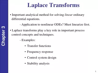
Laplace Transforms. Important analytical method for solving linear ordinary differential equations. - Application to nonlinear ODEs? Must linearize first. Laplace transforms play a key role in important process control concepts and techniques. - Examples: Transfer functions

Laplace Transforms
E N D
Presentation Transcript
Laplace Transforms • Important analytical method for solving linear ordinary • differential equations. • - Application to nonlinear ODEs? Must linearize first. • Laplace transforms play a key role in important process • control concepts and techniques. • - Examples: • Transfer functions • Frequency response • Control system design • Stability analysis
Definition The Laplace transform of a function, f(t), is defined as where F(s) is the symbol for the Laplace transform, L is the Laplace transform operator, and f(t) is some function of time, t. Note: The L operator transforms a time domain function f(t) into an s domain function, F(s). s is a complex variable: s = a + bj,
Inverse Laplace Transform, L-1: By definition, the inverse Laplace transform operator, L-1, converts an s-domain function back to the corresponding time domain function: Important Properties: Both L and L-1 are linear operators. Thus,
where: - x(t) and y(t) are arbitrary functions - a and b are constants - Similarly,
Laplace Transforms of Common Functions • Constant Function • Let f(t) = a (a constant). Then from the definition of the Laplace transform in (3-1),
Step Function • The unit step function is widely used in the analysis of process control problems. It is defined as: Because the step function is a special case of a “constant”, it follows from (3-4) that
Derivatives • This is a very important transform because derivatives appear in the ODEs we wish to solve. In the text (p.53), it is shown that initial condition at t = 0 Similarly, for higher order derivatives:
where: - n is an arbitrary positive integer - Special Case: All Initial Conditions are Zero Suppose Then In process control problems, we usually assume zero initial conditions. Reason: This corresponds to the nominal steady state when “deviation variables” are used, as shown in Ch. 4.
Exponential Functions • Consider where b > 0. Then, • Rectangular Pulse Function • It is defined by:
Time, t The Laplace transform of the rectangular pulse is given by
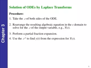
Impulse Function (or Dirac Delta Function) • The impulse function is obtained by taking the limit of the • rectangular pulse as its width, tw, goes to zero but holding • the area under the pulse constant at one. (i.e., let ) • Let, • Then, Solution of ODEs by Laplace Transforms • Procedure: • Take the L of both sides of the ODE. • Rearrange the resulting algebraic equation in the s domain to solve for the L of the output variable, e.g., Y(s). • Perform a partial fraction expansion. • Use the L-1 to find y(t) from the expression for Y(s).
Table 3.1. Laplace Transforms • See page 54 of the text.
Example 3.1 Solve the ODE, First, take L of both sides of (3-26), Rearrange, Take L-1, From Table 3.1,
Partial Fraction Expansions Basic idea: Expand a complex expression for Y(s) into simpler terms, each of which appears in the Laplace Transform table. Then you can take the L-1 of both sides of the equation to obtain y(t). Example: Perform a partial fraction expansion (PFE) where coefficients and have to be determined.
To find : Multiply both sides by s + 1 and let s = -1 To find : Multiply both sides by s + 4 and let s = -4 A General PFE Consider a general expression,
Here D(s) is an n-th order polynomial with the roots all being real numbers which are distinct so there are no repeated roots. The PFE is: Note:D(s) is called the “characteristic polynomial”. • Special Situations: • Two other types of situations commonly occur when D(s) has: • Complex roots: e.g., • Repeated roots (e.g., ) • For these situations, the PFE has a different form. See SEM • text (pp. 61-64) for details.
Example 3.2 (continued) Recall that the ODE, , with zero initial conditions resulted in the expression The denominator can be factored as Note: Normally, numerical techniques are required in order to calculate the roots. The PFE for (3-40) is
Solve for coefficients to get (For example, find , by multiplying both sides by s and then setting s = 0.) Substitute numerical values into (3-51): Take L-1 of both sides: From Table 3.1,
Important Properties of Laplace Transforms • Final Value Theorem It can be used to find the steady-state value of a closed loop system (providing that a steady-state value exists. Statement of FVT: providing that the limit exists (is finite) for all where Re (s) denotes the real part of complex variable, s.
Example: Suppose, Then, 2. Time Delay Time delays occur due to fluid flow, time required to do an analysis (e.g., gas chromatograph). The delayed signal can be represented as Also,