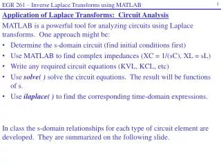
Application of Laplace Transforms: Circuit Analysis
130 likes | 815 Vues
EGR 261 – Inverse Laplace Transforms using MATLAB. Application of Laplace Transforms: Circuit Analysis MATLAB is a powerful tool for analyzing circuits using Laplace transforms. One approach might be: Determine the s-domain circuit (find initial conditions first)

Application of Laplace Transforms: Circuit Analysis
E N D
Presentation Transcript
EGR 261 – Inverse Laplace Transforms using MATLAB • Application of Laplace Transforms: Circuit Analysis • MATLAB is a powerful tool for analyzing circuits using Laplace transforms. One approach might be: • Determine the s-domain circuit (find initial conditions first) • Use MATLAB to find complex impedances (XC = 1/(sC), XL = sL) • Write any required circuit equations (KVL, KCL, etc) • Use solve( ) solve the circuit equations. The result will be functions of s. • Use ilaplace( ) to find the corresponding time-domain expressions. • In class the s-domain relationships for each type of circuit element are developed. They are summarized on the following slide.
EGR 261 – Inverse Laplace Transforms using MATLAB R R C 1/(sC) v(0)/s sL L Li(0) 10V 10/s 2mA 0.002/s s-domain circuit models time-domain s-domain
Lecture #22 EGR 267 – Engineering Analysis Tools • Procedure: Circuit Analysis using the Laplace-transformed Circuit • Draw the circuit at t = 0-. • Assume that the circuit is in steady state. • Draw inductors as short circuits and capacitors as open circuits. • Find vC(0-) and iL(0-) – these are needed for step 2. • Draw the s-domain circuit for t > 0. • Analyze the circuit as you might analyze a DC circuit (using any circuit analysis method). Recall that the s-domain impedances sL and 1/(sC) act essentially like resistors. Determine the desired result in the s-domain (V(s), I(s), etc). • Convert the result back to the time domain. In other words, use inverse Laplace transforms to find v(t) or i(t) from V(s) or I(s). • Note: If the circuit has zero initial conditions then the voltage sources in the capacitor and inductor models will be zero.
EGR 261 – Inverse Laplace Transforms using MATLAB + VC(t) _ 28 ohms 4 H + - 160 V 0.025 F Example 1: Use Laplace transforms and MATLAB to determine i(t) and vC(t) in the circuit shown below (for t > 0). Assume that all initial conditions are zero. i(t)
EGR 261 – Inverse Laplace Transforms using MATLAB Example 1 (continued)
EGR 261 – Inverse Laplace Transforms using MATLAB Example 2: Use Laplace transforms and MATLAB to determine ia(t) and ib(t) in the circuit shown below (for t > 0). Assume that all initial conditions are zero. ia(t) ib(t)
EGR 261 – Inverse Laplace Transforms using MATLAB Example 2 (continued)
EGR 261 – Inverse Laplace Transforms using MATLAB Example 3: (class example) Use Laplace transforms and MATLAB to determine i(t) and v(t) in the circuit shown below (for t > 0). Assume that vC(0) = 50V and i(0) = 100 mA. 8 mH 10 uF i(t) + v(t) - + - 336 V 4k 2k