Taylor Series
Taylor Series. SOLUTION OF NON-LINEAR EQUATIONS. All equations used in horizontal adjustment are non-linear. Solution involves approximating solution using 1'st order Taylor series expansion, and Then solving system for corrections to approximate solution.


Taylor Series
E N D
Presentation Transcript
SOLUTION OFNON-LINEAR EQUATIONS • All equations used in horizontal adjustment are non-linear. • Solution involves approximating solution using 1'st order Taylor series expansion, and • Then solving system for corrections to approximate solution. • Repeat solving system of linearized equations for corrections until corrections become small. • This process of solving equations is known as: ITERATING
Taylor’s Series Given a function, L = f(x,y)
Taylor’s Series • The series is also non-linear (unknowns are the dx’s, dy’s, and higher order terms) • Therefore, truncate the series after only the first order terms, which makes the equation an approximation • Initial approximations generally need to be reasonably close in order for the solution to converge
Solution • Determine initial approximations (closer is better) • Form the (first order) equations • Solve for corrections, dx and dy • Add corrections to approximations to get improved values • Iterate until the solution converges
Example C.1 Solve the following pair of non-linear equations. Use initial approximation of 1 (one) for both x and y. First, determine the partial derivatives
Write the Linearized Equations Simplify
Solve New approximations:
Linearized Equations – Iteration 2 Simplify
Solve – Iteration 2 New approximations:
Iteration 3 Same procedure yields: dx = 0.00 and dy = -0.11 This results in new approximations of x = 2.00 and y = 2.00 Further iterations are negligible
General Matrix Form • The coefficient matrix formed by the partial derivatives of the functions with respect to the variables is the Jacobian matrix • It can be used directly in a general matrix form
General Form for Example JX = K
Circle Example Determine the equation of a circle that passes through the points (9.4, 5.6), (7.6, 7.2), and (3.8, 4.8). Initial approximations for unknown and circle equation: Center point: (7, 4.5), Radius: 3 Rearranged Linearizing