Download
1 / 23
280 likes | 731 Vues
9.7 Taylor Series. Taylor Series. Brook Taylor was an accomplished musician and painter. He did research in a variety of areas, but is most famous for his development of ideas regarding infinite series. Brook Taylor 1685 - 1731. Identify this graph:. What if we zoom out a bit?.

E N D
Taylor Series Brook Taylor was an accomplished musician and painter. He did research in a variety of areas, but is most famous for his development of ideas regarding infinite series. Brook Taylor 1685 - 1731
Identify this graph: What if we zoom out a bit? And a bit more? What the?! The actual function is:
Suppose we wanted to find a fifth degree polynomial of the form: that approximates the behavior of at If we make , and the first, second, third, fourth, and fifth derivatives the same, then we would have a pretty good approximation.
0 1 0
0 1 0
-1 0 1
-1 0 1
P(x) is the fifth degree polynomial that has the same first through fifth derivatives at x = 0 that f(x) = sin x has. We call P(x) the 5th degree Taylor Polynomial of f(x) at x = 0.
If we plot both functions, we see that near zero the functions match very well!
This pattern occurs no matter what the original function was! Our polynomial: has the form: or: This is called a Taylor Polynomial. If we continue this pattern infinitely, we get a Taylor Series. When the series is centered at x = 0, it is called a Maclaurin Series.
Maclaurin Series: (generated by f at ) Taylor Series: (generated by f at ) If we want to center the series (and it’s graph) at some point other than zero, we get the Taylor Series:
Example: Generate the Maclaurin Series for The formula for Maclaurin Series is:
The 3rd order polynomial for is , but it is degree 2. When referring to Taylor polynomials, we can talk about number of terms, order or degree. This is a polynomial in 3 terms. It is a 4th order Taylor polynomial, because it was found using the 4th derivative. It is also a 4th degree polynomial, because x is raised to the 4th power. The x3 term drops out when using the third derivative. A recent AP exam required the student to know the difference between order and degree. This is also the 2nd order polynomial.
A Taylor Polynomial is used to approximate a function. A Taylor Series is equal to a function.
In practice, we usually use a Taylor Polynomial to approximate a function so we also want to know the error in using the approximation. The error (also known as the remainder, Rn(x)) is the difference between the actual value of the function, f(x), and the polynomial of degree n, Pn(x).
Taylor’s Theorem specifies that the remainder Rn(x) (also called the Lagrange Error or Lagrange form of the remainder) is given by the formula: z This looks a lot like the next term in the Taylor Series except that it is not evaluated at a but at some number z which is between x and a. z
Taylor’s Theorem guarantees that there exists a value of z between a and x such that: It usually isn’t possible to find the value of but you can often find an upper bound on it. This will be called max
Example: Therefore the Lagrange error term