Bayesian networks Variable Elimination
680 likes | 736 Vues
Learn about compact representations of probability distributions, automated probabilistic inference, likelihood queries, a posteriori beliefs, MAP queries, and complexity of inference.

Bayesian networks Variable Elimination
E N D
Presentation Transcript
BayesiannetworksVariable Elimination Based on Nir Friedman’s course (Hebrew University) Automated Planning and Decision Making 2007
In previous lessons we introduced compact representations of probability distributions: • Bayesian Networks • A network describes a unique probability distribution P • How do we answer queries about P? • The process of computing answers to these queries is called probabilistic inference Automated Planning and Decision Making
Queries: Likelihood • There are many types of queries we might ask. • Most of these involve evidence • An evidence e is an assignment of values to a set E of variables in the domain • Without loss of generality E = { Xk+1, …, Xn } • Simplest query: compute probability of evidence • This is often referred to as computing the likelihood of the evidence Automated Planning and Decision Making
Queries: A posteriori belief • Often we are interested in the conditional probability of a variable given the evidence • This is the a posteriori belief in X, given evidence e • A related task is computing the term P(X, e) • i.e., the likelihood of e and X = x for values of X • we can recover the a posteriori belief by Automated Planning and Decision Making
A posteriori belief This query is useful in many cases: • Prediction: what is the probability of an outcome given the starting condition • Target is a descendent of the evidence • Diagnosis: what is the probability of disease/fault given symptoms • Target is an ancestor of the evidence • As we shall see, the direction between variables does not restrict the directions of the queries • Probabilistic inference can combine evidence form all parts of the network Automated Planning and Decision Making
Queries: A posteriori joint • In this query, we are interested in the conditional probability of several variables, given the evidenceP(X, Y, … | e ) • Note that the size of the answer to query is exponential in the number of variables in the joint Automated Planning and Decision Making
Queries: MAP • In this query we want to find the maximum a posteriori assignment for some variable of interest (say X1,…,Xl ) • That is, x1,…,xl maximize the probabilityP(x1,…,xl | e) • Note that this is equivalent to maximizingP(x1,…,xl, e) Automated Planning and Decision Making
Queries: MAP We can use MAP for: • Classification • find most likely label, given the evidence • Explanation • What is the most likely scenario, given the evidence Automated Planning and Decision Making
Queries: MAP Cautionary note: • The MAP depends on the set of variables • Example: • MAP of X is 1, • MAP of (X, Y) is (0,0) Automated Planning and Decision Making
Complexity of Inference Theorem: Computing P(X = x) in a Bayesian network is NP-hard Not surprising, since we can simulate Boolean gates. Automated Planning and Decision Making
Proof We reduce 3-SAT to Bayesian network computation Assume we are given a 3-SAT problem: • q1,…,qn be propositions, • 1 ,... ,k be clauses, such that i = li1 li2 li3 where each lij is a literal over q1,…,qn • = 1... k We will construct a network s.t. P(X=t) > 0 iff is satisfiable Automated Planning and Decision Making
... P(Qi = true) = 0.5, P(I = true| Qi , Qj , Ql ) = 1 iff Qi , Qj , Qlsatisfy the clause I A1, A2, …, are simple binary and gates Q1 Q2 Q3 Q4 Qn ... k-1 1 2 3 k ... A1 A2 X Ak/2-1 Automated Planning and Decision Making
It is easy to check • Polynomial number of variables • Each CPDs can be described by a small table (8 parameters at most) • P(X = true) > 0 if and only if there exists a satisfying assignment to Q1,…,Qn • Conclusion: polynomial reduction of 3-SAT Automated Planning and Decision Making
Note: this construction also shows that computing P(X = t) is harder than NP • 2nP(X = t) is the number of satisfying assignments to • Thus, it is #P-hard (in fact it is #P-complete) Automated Planning and Decision Making
Hardness - Notes • We used deterministic relations in our construction • The same construction works if we use (1-, ) instead of (1,0) in each gate for any < 0.5 • Hardness does not mean we cannot solve inference • It implies that we cannot find a general procedure that works efficiently for all networks • For particular families of networks, we can have provably efficient procedure Automated Planning and Decision Making
Inference in Simple Chains How do we compute P(X2)? X1 X2 Automated Planning and Decision Making
Inference in Simple Chains (cont.) How do we compute P(X3)? • we already know how to compute P(X2)... X1 X2 X3 Automated Planning and Decision Making
Xn X1 X2 X3 Inference in Simple Chains (cont.) ... How do we compute P(Xn)? • Compute P(X1), P(X2), P(X3), … • We compute each term by using the previous one Complexity: • Each step costs O(|Val(Xi)|*|Val(Xi+1)|) operations • Compare to naïve evaluation, that requires summing over joint values of n-1 variables Automated Planning and Decision Making
Inference in Simple Chains (cont.) • Suppose that we observe thevalue of X2 =x2 • How do we compute P(X1|x2)? • Recall that it suffices to compute P(X1,x2) X1 X2 Automated Planning and Decision Making
Inference in Simple Chains (cont.) • Suppose that we observe the value of X3 =x3 • How do we compute P(X1,x3)? • How do we compute P(x3|x1)? X1 X2 X3 Automated Planning and Decision Making
Variable Elimination General idea: • Write query in the form • Iteratively • Move all irrelevant terms outside of innermost sum • Perform innermost sum, getting a new term • Insert the new term into the product Automated Planning and Decision Making
Smoking Visit to Asia Tuberculosis Lung Cancer Abnormality in Chest Bronchitis Dyspnea X-Ray A More Complex Example • “Asia” network: Automated Planning and Decision Making
We want to compute P(d) • Need to eliminate: v,s,x,t,l,a,b Initial factors S V L T B A X D Automated Planning and Decision Making
Compute: S V L T B A • We want to compute P(d) • Need to eliminate: v,s,x,t,l,a,b • Initial factors X D Eliminate: v Note: fv(t) = P(t) In general, result of elimination is not necessarily a probability term Automated Planning and Decision Making
S V L T B A X D Compute: • We want to compute P(d) • Need to eliminate: s,x,t,l,a,b • Initial factors Eliminate: s Summing on s results in a factor with two arguments fs(b,l) In general, result of elimination may be a function of several variables Automated Planning and Decision Making
S V L T B A X D Compute: • We want to compute P(d) • Need to eliminate: x,t,l,a,b • Initial factors Eliminate: x Note: fx(a) = 1 for all values of a !! Automated Planning and Decision Making
S V L T B A X D Compute: • We want to compute P(d) • Need to eliminate: t,l,a,b • Initial factors Eliminate: t Automated Planning and Decision Making
S V L T B A X D Compute: • We want to compute P(d) • Need to eliminate: l,a,b • Initial factors Eliminate: l Automated Planning and Decision Making
S V L T B A X D å å f ( b , d ) f ( a , b ) f ( a ) p ( d | a , b ) f ( d ) f ( b , d ) = = a x a b l b • We want to compute P(d) • Need to eliminate: b • Initial factors Eliminate: a,b Compute: a Automated Planning and Decision Making
Variable Elimination • We now understand variable elimination as a sequence of rewriting operations • Actual computation is done in elimination step • Computation depends on order of elimination • We will return to this issue in detail Automated Planning and Decision Making
S V L T B A X D Dealing with evidence • How do we deal with evidence? • Suppose get evidence V = t, S = f, D = t • We want to compute P(L, V = t, S = f, D = t) Automated Planning and Decision Making
S V L T B A X D Dealing with Evidence • We start by writing the factors: • Since we know that V = t, we don’t need to eliminate V • Instead, we can replace the factors P(V) and P(T|V) with • These “select” the appropriate parts of the original factors given the evidence • Note that fp(V) is a constant, and thus does not appear in elimination of other variables Automated Planning and Decision Making
S V L T B A X D Dealing with Evidence • Given evidence V = t, S = f, D = t • Compute P(L, V = t, S = f, D = t ) • Initial factors, after setting evidence: Automated Planning and Decision Making
S V L T B A X D Dealing with Evidence • Given evidence V = t, S = f, D = t • Compute P(L, V = t, S = f, D = t ) • Initial factors, after setting evidence: • Eliminating x, we get Automated Planning and Decision Making
S V L T B A X D Dealing with Evidence • Given evidence V = t, S = f, D = t • Compute P(L, V = t, S = f, D = t ) • Initial factors, after setting evidence: • Eliminating x, we get • Eliminating t, we get Automated Planning and Decision Making
S V L T B A X D Dealing with Evidence • Given evidence V = t, S = f, D = t • Compute P(L, V = t, S = f, D = t ) • Initial factors, after setting evidence: • Eliminating x, we get • Eliminating t, we get • Eliminating a, we get Automated Planning and Decision Making
S V L T B A X D Dealing with Evidence • Given evidence V = t, S = f, D = t • Compute P(L, V = t, S = f, D = t ) • Initial factors, after setting evidence: • Eliminating x, we get • Eliminating t, we get • Eliminating a, we get • Eliminating b, we get Automated Planning and Decision Making
Complexity of variable elimination • Suppose in one elimination step we compute This requires • multiplications • For each value for x, y1, …, yk, we do m multiplications • additions • For each value of y1, …, yk , we do |Val(X)| additions Complexity is exponential in number of variables in the intermediate factor. Automated Planning and Decision Making
Understanding Variable Elimination • We want to select “good” elimination orderings that reduce complexity • We start by attempting to understand variable elimination via the graph we are working with • This will reduce the problem of finding good ordering to a graph-theoretic operation that is well-understood Automated Planning and Decision Making
Undirected graph representation • At each stage of the procedure, we have an algebraic term that we need to evaluate • In general this term is of the form: • where Zi are sets of variables • We now plot a graph where there is undirected edge X--Y if X,Y are arguments of some factor • that is, if X,Y are in some Zi Automated Planning and Decision Making
Undirected Graph Representation • Consider the “Asia” example • The initial factors are • thus, the undirected graph is • In the first step this graph is just the moralized graph S V S V L T L T B A B A X D X D Automated Planning and Decision Making
Undirected Graph Representation • Now we eliminate t, getting • The corresponding change in the graph is S S V V L L T T B B A A X D X D Automated Planning and Decision Making
S V L T B A X D Example • Want to computeP(L, V = t, S = f, D = t) • Moralizing S V L T B A X D Automated Planning and Decision Making
S V L T B A X D Example • Want to computeP(L, V = t, S = f, D = t) • Moralizing • Setting evidence S V L T B A X D Automated Planning and Decision Making
S V L T B A X D Example • Want to computeP(L, V = t, S = f, D = t) • Moralizing • Setting evidence • Eliminating x • New factor fx(A) S V L T B A X D Automated Planning and Decision Making
S V L T B A X D Example • Want to computeP(L, V = t, S = f, D = t) • Moralizing • Setting evidence • Eliminating x • Eliminating a • New factor fa(b,t,l) S V L T B A X D Automated Planning and Decision Making
S V L T B A X D Example • Want to computeP(L, V = t, S = f, D = t) • Moralizing • Setting evidence • Eliminating x • Eliminating a • Eliminating b • New factor fb(t,l) S V L T B A X D Automated Planning and Decision Making
S V L T B A X D Example • Want to computeP(L, V = t, S = f, D = t) • Moralizing • Setting evidence • Eliminating x • Eliminating a • Eliminating b • Eliminating t • New factor ft(l) S V L T B A X D Automated Planning and Decision Making
Elimination in Undirected Graphs • Generalizing, we see that we can eliminate a variable x by 1. For all Y,Z, s.t., Y--X, Z--X • add an edge Y--Z 2. Remove X and all adjacent edges to it • This procedure creates a clique that contains all the neighbors of X • After step 1 we have a clique that corresponds to the intermediate factor (before marginalization) • The cost of the step is exponential in the size of this clique Automated Planning and Decision Making
Undirected Graphs • The process of eliminating nodes from an undirected graph gives us a clue to the complexity of inference • To see this, we will examine the graph that contains all of the edges we added during the elimination. The resulting graph is always chordal. Automated Planning and Decision Making
