Download
1 / 47
470 likes | 610 Vues
This workshop covers the fundamental aspects of interest rate mathematics, including definitions, key concepts, and various calculations for different types of interest, including simple and compound interest. It explores essential assumptions such as annualization, compounding frequency, and the time value of money. Participants will gain insights into pricing discount instruments, holding period yield, and the features of bonds. The workshop aims to provide a comprehensive understanding of interest rate calculations essential for finance and investment professionals.

E N D
Workshop On Interest Rate Mathematics
I • Interest Rates • The interest rate is the amount paid by the borrower to the lender for the use of the lender’s funds. • Two major assumptions / conventions used in calculating interest rates and rates of return are the, • per annum standardization and • number of compounds
Per Annum Normalization The most obvious of the interest rate conventions is that interest rates are quoted on a nominal per annum basis (p.a.). Compound Period A compound period is a length of time at the end of which interest earned is capitalized.
t Frequency of Compounding The numerical value of an interest rate is dependent upon an assumption as to frequency of compounding. For example, the growth of a sum of Rs.1000 to Rs.2000 over one year can be expressed as a rate of interest of, 100.00% simple interest 82.84% semi-annual compounding 71.36% monthly compounding 69.78% weekly compounding
t Frequency of Compounding One important property of compound interest is that the future value increases with the frequency of compounding. However, the rate of increase of future value decreases as the frequency of compounding increases.
Time Value of Money The time value of money is represented by the growth of an invested sum. The growth of Rs.1000 to Rs.2000 over a year reveals the value that lenders and borrowers place on time. The increase of Rs.1000 indicates the time value of money. By convention we express the time value of money as an interest rate per annum. The exact numerical value for the interest rate implied by the time value of money is entirely dependent upon the assumed frequency of compounding.
Simple Interest Under simple interest, the interest received is proportional to the principal invested and to the time that the funds remain invested. FV = PV ( 1 + r t ) We can turn the simple interest equation around to show the interest rate on a simple interest investment. r = ( FV / PV ) * 1/t
si Pricing Discount Instruments These securities do not provide their holder with an explicit interest payment. In order for the holder to receive the equivalent of an interest payment these securities are sold at price PV, for less than their face value FV, this being the amount repaid by the lender on the security’s maturity date. PV = FV / ( 1 + r t )
Holding Period Yield • Not all investments actually achieve the yield to maturity, because securities are often sold before they mature. In these cases the investment yield is a holding period yield (HPY). It contains two components. • nominal yield • capital gains/losses • Computation • r = [ Psell / Pbuy – 1 ] / t
Forward Interest Rate Forward Rate = (1 +Li x Lt)– 1 x __365_ (1+Si x St) (Lt – St) Where, Li = Long Tenor Interest Rate Si = Short Tenor Interest Rate Lt = Long Tenor St = Short Tenor • Short Term Yield Curve
Compound Interest Compound interest means that the interest adds to the principal and thus in the next period interest is calculated on the principal, plus the previous period’s interest. FV = PV 1 + i/n t*n Where FV = Future Value PV = Present Value i = Interest Rate per annum n = Number of compounds per year t = Time in years
Bond’s and Their Pricing • A bond is a financial instrument consisting of a contract to pay, • a fixed sum called the face value at a given future date, called maturity date or redemption date, and • a series of equal periodic payments called interest payments.
t Compound Interest The present value and the compound period holding period yield or interest rate can be found by simply rearranging the compound interest equation. PV = . FV . 1 + i/n t*n i = (FV/PV)1/t*n – 1 n
The Basic Features Of A Bond • A bond is characterized by , • its denomination or face value, for example PKR 100 Million; • its maturity date, for example, 24-Oct-2012; • its coupon rate, for example 10.00% p.a. • the frequency of coupon payments per year and the specific dates of each payment; and • identification of the issuer.
Bond Pricing • The price of a bond is simply the sum of the present value of the future cash flows. • Interest rates on a multi-payment instrument, such as an annuity or bond, are assumed to assumed compound at the same frequency as the cash payments are made. If payments are made quarterly the instrument is priced using yields computed on a quarterly compound basis. If payments are made semi-annually, the instrument is priced using semi-annual yields. P = C 1 + C 2 + …………. + (100 + Cn) (1+i) (1+i)2 (1+i)n
Annuity • An annuity is a sequence of regular periodic payments. • Commonly occurring examples of Annuities are premiums on insurance policies, interest payments on bonds and debentures, lease and rental payments, and most loan payments.
Present Value of an Annuity • a n|i = 1 – (1+i)-n i • A bond’s coupon payments form an annuity, thus the value of any bond is given as the present value of this annuity added to the discounted amount of the face value. P = C a n|i + F . (1+i)n Where, P refers to the bond’s price F is the Rupee redemption value C is the coupon amount i is the yield to maturity per compound period and n is the number of interest periods
Accumulation of Interest • Between the coupon dates a bond conceptually accumulates interest. For broken period bonds calculate the present value till the next coupon date and then discount the value to the current date. This value will include the accrued interest, which needs to be adjusted to arrive at the clean price. P = Discount Value – Accrued Interest Discount Value = 1 . f/d C (1 + a n|i) + . F . 1+i (1+i)n
Accumulation of Interest Accrued Interest = C * (d – f) d Where, f is the number of days to next interest date and d is the number of days in the current interest interval
Term Structure of Interest Rates • Term structure analysis focuses on the relationship between the interest rate attached to an investment and the term of the investment. A security will however, only have an unambiguous length if it makes a single payment at time, t.
Term Structure of Interest Rates • The ambiguity in the relationship between the yield on coupon bonds and their term may be rectified by estimating the underlying zero coupon yields from the coupon bond yields by conceptually stripping off coupons. In this method coupons are sequentially “stripped” from a bond to reveal the underlying implied zero coupon rate.
Term Structure of Interest Rates • There are four ways to describe any term structure shape. In each case one of four alternative variables is set out against the term. The four alternative variables are, • spot zero coupon interest rates, • forward interest rates, • discount factors and • cumulative sums.
Term Structure of Interest Rates • Each of these variables are alternative to each other. Each contains the same information and one variable can always be obtained from any other variable. In most cases there is no adequate market for zero coupon instruments hence the term structure must be implied from the yields on coupon bonds. • The first step in the production of a term structure is to construct a par curve, that is a set of yields on par bonds. A par bond’s coupon rate is equal to the yield and as a consequence the price of a par bond is Rs. 100 per Rs. 100 of face value
Deriving a Set of Discount Factors • A discount factor is a figure that converts a cash flow in a future period back to the present. • The value of a bond is simply the sum of its cash flows multiplied by their appropriate discount factors. Thus for a par bond paying a Rs. C per period the following equation holds • 100 = C*d1 + C*d2 + …………….. (C+100)*dn
Deriving a Set of Discount Factors This provides us with simple method for sequentially computing discount factors as, dn = 100 – C (d1 + d2 + ……..dn) C + 100 If we know the first discount factor we can sequentially deduce the rest.
Cumulative Sum The cumulative sum is the inverse of the discount factor. The cumulative sum converts a present value to a future value. FVi = PV*CSi Where CSi is the cumulative sum. The cumulative sum represents the proceeds of an investment made for i periods. The cumulative sum may be standardized on any starting sum.
Zero Coupon Rates The zero coupon rates are easily computed from the cumulative sum series. The zero coupon rate, for a particular term, is that rate implied by the growth of an investment over that period. Zero rates may be calculated from either the cumulative sum or the discount factors, R = CSt1/2t - 1 CSo = do. 1/2t - 1 dt
Forward Rates • Finally the term structure may be represented by a series of forward rates. A forward interest rate is a rate on a security that begins its life a time in the future. As the term structure is normally drawn on the basis of semi-annual compounding, the forward rate curve normally plots six month forward rates. • Forward rates are easily computed from adjacent cumulative sums f = CFt. – 1 * 2 CFt-1
Interest Rate Risk and Duration • The holder of a bond will realize the purchase yield if, • the bond is held to maturity and • all coupons are reinvested at the purchase yield. • Changes in yields impinge upon fixed interest returns in two ways. • reduce the value of bonds and result in capital losses should bonds have to be liquidated prior to maturity. This is called price risk. • reduce the value of reinvested coupons. This is called reinvestment risk.
Price RiskAs interest rates rise, asset values fall. However the extent of the fall depends upon the nature of the asset.Consider the reaction of three bonds as yields rise from 10%p.a. to 12%p.a.
The above table illustrates two general principals of the sensitivity of a bond to change in yields. • the price of low coupon bonds are more sensitive to a given change in market yields than the prices of high coupon bonds; and • the price of longer tenor bonds are more sensitive to changes in yields than the prices of shorter maturity bonds.
Duration Duration is a measure of the average time at which payments are made. While duration is commonly applied to bonds, the concept is applicable to any cash flow. Duration is measured not as a simple average of the time of payments but as a weighted average. The timing of payments are weighted by the present value of those payments.
Duration in this case is lower than the maturity is a consequence of the coupon payments made prior to maturity. • The only bond with a duration equal to its tenor is a zero-coupon bond whose only payment occurs at maturity.
Measurement of Price Sensitivity • Duration as a measure of the average time of payment is viewed as a measure of the effective length of life of a security but it is not the principal reason for its use in finance. • Duration is mostly used as a measure of a security’s price sensitivity to changes in interest rates. • This use is a direct result of there being, for a coupon paying bond, a relationship between, • duration; and • the percentage change in the bond’s value caused by a change in interest rates.
Modified Duration Modified duration provides a measure of the sensitivity of an instrument to small parallel changes in interest rates. Specifically, D! = D / 1 + i The left hand side of the above equation is the percentage change in the price of an asset is approximately equal –D! for every 1% change in yields. The modified duration of the 3 year 10% bond is, D! = 2.66 / 1.05 = 2.54 years
Modified duration predicted price changes will be accurate only for small and parallel changes in the yield curve owing to curvilinear nature of the relationship between price and yield. • Duration Properties • Duration is able to function as a measure of sensitivity because all other things being equal a bond’s duration will be greater: • the smaller the coupon payments relative to the redemption value. • the lower is yield and • the greater the time to redemption
Asset / Liability Management Interest rate movements affect the value of both assets and liabilities. If an interest rate change induces a different change in the of liabilities to that of assets then the balance sheet is exposed to interest rate risk. A way a firm can measure its exposure to interest rate risk is to estimate the difference between the modified duration of its assets and liabilities.
Convexity Convexity concerns itself with changes in the slope of the bond price line. It provides a second order correction to bond sensitivity equation. Convexity can be expressed as, C = D!2 + D / 2 1+ i Convexity, by adding another term, increases the accuracy of the bond sensitivity equation. ΔP = D! Δr + ½ C Δr² P
The duration, D = ∑t*PV / Price = 425.0780 / 107.7217 = 3.9461 years Modified Duration, D! = D / (1+i) = 3.9461 / 1.05 = 3.7582 years D2 = ∑ t²*PV / Price = 1930.3570 / 107.7217 = 17.9198 years² D2! = D2 / (1+i) = 17.9189 / 1.05 = 17.0665 years²
The bond’s convexity, C is computed from C = (D!2 + D!/2) / (1 + I) = (17.0665 + 3.7582/2) / 1.05 = 18.0434
Barber’s Approximation • Barber approximated the percentage change by a Taylor series expansion of the natural log of price, ΔP = exp -D! Δr + ½ (C – D!²)(Δr)² - 1 P
Convexity Properties • For any given yield and coupon the longer the tenor of bond the greater the convexity. • For any given yield and maturity, the greater the coupon the smaller the convexity. • For any given coupon and maturity, the higher the yield, the smaller the convexity. • For any given duration the higher the coupon the higher the convexity. • The bond with larger convexity will appreciate more when yields decline and less when yields rise.