Neutral Stability
Chapter 6. The Frequency-Response Design Method. Neutral Stability. Root-locus technique determine the stability of a closed-loop system, given only the open-loop transfer function KG ( s ), by inspecting the denominator in factored form.

Neutral Stability
E N D
Presentation Transcript
Chapter 6 The Frequency-Response Design Method Neutral Stability • Root-locus technique determine the stability of a closed-loop system, given only the open-loop transfer function KG(s), by inspecting the denominator in factored form. • Frequency response technique determine the stability of a closed-loop system, given only the open-loop transfer function KG(jω) by evaluating it and performing a test on it. The principle will be discussed now.
Chapter 6 The Frequency-Response Design Method Neutral Stability • Suppose we have a system defined by • System is unstable if K > 2. • The neutrally stable points lie on the imaginary axis, K = 2 and s = ±j. • All points on the locus fulfill:
Chapter 6 The Frequency-Response Design Method Neutral Stability • The frequency response of the system for various values of K is shown as follows. • At K = 2, the magnitude response passes through 1 at the frequency ω = 1 rad/sec (remember s = ±j), at which the phase passes through 180°. • After determining “the point of neutral stability”, we know that: • K < Kneutral stability stable, • K > Kneutral stability unstable. • At (ω = 1 rad/sec, G(jω) = –180°), • |KG(jω)| < 1 stable K, • |KG(jω)| > 1 unstable K.
Chapter 6 The Frequency-Response Design Method Neutral Stability • A trial stability condition can now be stated as follows • If |KG(jω)|< 1 at G(jω) = –180°, • then the system is stable. • This criterion holds for all system for which increasing gain leads to instability and|KG(jω)| crosses magnitude=1 once. • For systems where increasing gain leads from instability to stability, the stability condition is • If |KG(jω)|> 1 at G(jω) = –180°, • then the system is stable. • For other more complicated cases, the Nyquist stability criterion can be used, which will be discussed next. • While Nyquist criterion is fairly complex, one should bear in mind, that for most systems a simple relationship exists between the closed-loop stability and the open-loop frequency response. “ ” “ ”
Chapter 6 The Frequency-Response Design Method The Nyquist Stability Criterion • The Nyquist stability criterion is based on the argument principle. • It relates the open-loop frequency response KG(s)to the number of closed-loop poles of the system (roots of the characteristic equation 1+ KG(s))that are in the RHP. • It is useful for stability analysis of complex systems with more than one resonance where the magnitude curve crosses 1 several times and/or the phase crosses 180° several times. • Advantage: From the open-loop frequency response (in the form of Bode plot), we can determine the stability of the closed-loop system without the need to determine the closed-loop poles.
Chapter 6 The Frequency-Response Design Method The Nyquist Stability Criterion • Consider the transfer function H1(s) with poles and zeros as indicated in the s-plane in (a) below. • We wish to evaluate H1 for values of s on the clockwise contour C1, with s0 as test point, • As s travels along C1 in the clockwise direction starting at s0, the angle α increases and decreases, and finally returns to the original value as s returns to s0, without rotating through 360°, see (b).
Chapter 6 The Frequency-Response Design Method The Nyquist Stability Criterion • α changes, but did not undergo a net change of 360° because there are no poles or zeros within C1. • Thus, none of the angles θ1, θ2, Φ1, or Φ2 go through a net revolution. • Since there is no net revolution, the plot of H1(s) in (b) will not encircle the origin. • Magnitude of H is equivalent to distance from origin to s0 • Phase of H is equivalent to α
Chapter 6 The Frequency-Response Design Method The Nyquist Stability Criterion • Now, consider the transfer function H2(s) with poles and zeros as indicated in the s-plane in (c). • We wish to evaluate H2 for values of s on the clockwise contour C1, noting that there is a pole within C1. • As s travels in the clockwise direction around C1, the contributions from θ1, θ2, and Φ1 change, but return to their original values as s returns to s0. • In contrast, Φ2 undergoes a net change of –360° after one full trip around C1 H2 encircles the origin in ccw direction.
Chapter 6 The Frequency-Response Design Method The Nyquist Stability Criterion • The essence of the argument principle: • A contour map of a complex function will encircle • the origin Z – P times, where Z is the number • of zeros and Pis the number of poles of • the function inside the contour. “ ”
Chapter 6 The Frequency-Response Design Method Application to Control Design • To apply the argument principle to control design, we let the contour C1 to encircle the entire RHP in the s-plane. • As we know, RHP is the region in the s-plane where a pole would cause an unstable system. • The resulting evaluation of H(s) will encircle the origin only if H(s) has a RHP pole or zero.
Chapter 6 The Frequency-Response Design Method Application to Control Design • As the stability is decided by the roots of the characteristic equation 1+KG(s), the argument principle must be applied to the function 1+KG(s). • If the evaluation contour, which encloses the entire RHP of the s-plane, contains a zero or pole of 1+KG(s), then the evaluated argument of 1+KG(s) will encircle the origin. • Furthermore, if the argument of 1+KG(s) encircles the origin, then it is equivalent with if the argument of KG(s) encircles –1 on the real axis. ≡
Chapter 6 The Frequency-Response Design Method Application to Control Design • Therefore, we can plot the contour evaluation of the open-loop KG(s), examine its encirclements of –1, and draw the conclusions about the origin encirclements of the closed-loop functions 1+KG(s). • Presentation of the argument evaluation of KG(s) in this manner is often referred to as a Nyquist plot, or polar plot. ≡
Chapter 6 The Frequency-Response Design Method Application to Control Design • 1+KG(s) is now written in terms of poles and zeros of KG(s), • The poles of 1+KG(s) are also the poles of G(s) • The poles of closed-loop transfer function are also the poles of the open-loop transfer function. • It is safe to assume that the poles of G(s) are known. • Since in most of the cases, the open-loop stability can be inspected in advance. • The zeros of 1+KG(s) are roots of the characteristic equation • If any of these zeros lies in the RHP, then the system will be unstable. • An encirclement of –1 by KG(s)or,equivalently,an encirclement of 0 by 1+KG(s) indicates a zero of 1+KG(s) in the RHP, and thus an unstable root of the closed-loop system.
Chapter 6 The Frequency-Response Design Method Application to Control Design • This basic idea can be generalized by noting that: • A clockwise contour C1 enclosing a zero of 1+KG(s)—that is, an unstable closed-loop pole— will result in KG(s) encircling the –1 point in a clockwise direction. • A clockwise contour C1 enclosing a pole of 1+KG(s)—that is, an unstable open-loop pole— will result in KG(s) encircling the –1 point in a counter-clockwise direction. • Furthermore, if two poles or two zeros are in the RHP, KG(s) will encircle –1 twice, and so on. • The net number of clockwise encirclements,N, equals the number of zeros in the RHP, Z, minus the number of open-loop poles in the RHP, P.
Chapter 6 The Frequency-Response Design Method Application to Control Design • Procedure for Plotting the Nyquist Plot: • Plot KG(s) for –j∞≤s≤+j∞. Do this by first evaluating KG(jω) for ω=0 to ω=+∞, which is exactly the frequency response of KG(jω). Since G(–jω) is the complex conjugate of G(jω), the evaluation for ω=0 to ω=–∞ can be obtained by reflecting the 0≤s≤+j∞ portion about the real axis. The Nyquist plot will always be symmetric with respect to the real axis. • Evaluate the number of clockwise encirclements of –1, and call that number N. If encirclements are in the counterclockwise direction, N is negative. • Determine the number of unstable (RHP) poles of G(s), and call that number P. • Calculate the number of unstable closed-loop roots Z: Z=N+P. If the system is stable, then Z = 0; that is, no characteristic equation roots in the RHP
Chapter 6 The Frequency-Response Design Method Application to Control Design Root locus of G(s) = 1/(s+1)2 Bode plot for KG(s) = 1/(s+1)2, K = 1
Chapter 6 The Frequency-Response Design Method Application to Control Design • Nyquist plot of the evaluation of KG(s) = 1/(s+1)2. • The evaluation contour is C1, with K = 1. • No value of K would cause the plot to encircle –1 (N = 0). • No poles of G(s) in the RHP (P = 0). • The closed-loop system is stable for all K > 0 (Z = N + P = 0). Bode plot for KG(s) = 1/(s+1)2, K = 1
Chapter 6 The Frequency-Response Design Method Application to Control Design Root locus of G(s) = 1/[s(s+1)2] Bode plot for KG(s) = 1/[s(s+1)2], K = 1
Chapter 6 The Frequency-Response Design Method Application to Control Design II I • If there is a pole on the imaginary axis, the C1 contour can be modified to take a small detour around the pole to the right. • The contour is now divided into 4 sections, I-II, II-III, III-IV, and IV-I. IV III
Chapter 6 The Frequency-Response Design Method Application to Control Design • Evaluation of path I-II can be obtained from the Bode plot, corresponds to the frequency response of KG(jω) for K = 1 and ω=0 to ω=+∞. II I
Chapter 6 The Frequency-Response Design Method Application to Control Design • Nyquist plot is nothing but the polar magnitude of G(jω). • As the frequency traverses from ω=0 to ω=+∞, the corresponding magnitude and phase is plotted on the polar coordinate.
Chapter 6 The Frequency-Response Design Method Application to Control Design • At ω = 0–, G(jω) is asymptotic at –2 – j∞. • At ω = +∞, G(jω) is asymptotic at 0– + j0+. • Plotting G(jω) for ω=0 to ω=+∞ can be performed by plotting the complex coordinate given by the last equation for several frequencies.
Chapter 6 The Frequency-Response Design Method Application to Control Design • Evaluation of path III-IV is the reflection of Path I-II about the real axis. • We know that this path corresponds to the frequency response of KG(jω) for K=1 and ω=0 to ω=–∞. IV III
Chapter 6 The Frequency-Response Design Method Application to Control Design • Path II-III is a half circle with a very large radius, routing from positive imaginary axis to negative imaginary axis in clockwise direction. • This path can be evaluated by replacing R : very large number r : very small number II • Performing it, III • Evaluation of G(s) forms a 1.5-circle with a very small radius. • Inserting the value of θ, the circle starts at –270° and ends at 270°, routing in ccw direction.
Chapter 6 The Frequency-Response Design Method Application to Control Design • Path IV-I is a half circle with a very small radius, routing from negative imaginary axis to positive imaginary axis in counterclockwise direction. • This path can be evaluated by replacing • Performing it, • Evaluation of G(s) forms a half circle with a very large radius. • Inserting the value of θ, the half circle starts at 90° and ends at –90°, routing in clockwise direction.
Chapter 6 The Frequency-Response Design Method Application to Control Design IV • Combining all four sections, we will get the complete Nyquist plot of the system. II III I
Chapter 6 The Frequency-Response Design Method Application to Control Design • The plot crosses the real axis at ω=1 at –0.5. • No unstable poles of G(s), P=0. • No encirclement of –1, N=0. Z=N+P=0 → the system is stable. • If K>2, the plot will encircle –1 twice in cw direction, N=2. • Z=N+P=2 → the system is unstable with 2 roots in RHP.
Chapter 6 The Frequency-Response Design Method Homework 9 Draw the Nyquist Plot for Choose K=1. Based on the plot, determine the range of K for which the system is stable. Hint: Get representative frequency points before you sketch the Nyquist plot. The easiest way is to choose them is to choose: • The 10n points (0.001, 0.001, …, 1, 10, 100, …) • The break points ωb • The points of corrections, 1/5ωb and 5ωb • Due: Wednesday, 04.12.2013.