Download
1 / 34
340 likes | 504 Vues
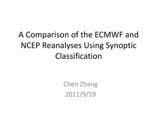
A Comparison of the ECMWF and NCEP Reanalyses Using Synoptic Classification. Chen Zhang 2011/9/19. Motivation. Why do we compare the reanalyses ? What do we want to know from the comparison? Synoptic scale Cloud parameterization How do we compare? Synoptic classification

E N D
A Comparison of the ECMWF and NCEP ReanalysesUsing Synoptic Classification Chen Zhang 2011/9/19
Motivation • Why do we compare the reanalyses? • What do we want to know from the comparison? • Synoptic scale • Cloud parameterization • How do we compare? • Synoptic classification • Cloud data associated • Correspondence in time series • Cloud structures • meteorology
Method • Initial clustering: sort atmospheric patterns into classes using basic variables • Resulting states can be interpreted in a number of ways: • recurring weather patterns • a collection of similar events • the average of the atmospheric variables across the cluster
Example of 2D clustering Courtesy Stuart Evans
Example of 2D clustering Courtesy Stuart Evans
Example of 2D clustering Courtesy Stuart Evans
Method • Improving cluster quality • A certain number of states is required in the initial clustering • Use cloud occurrence data associated with each state to perform two statistical tests of quality • Stability: are the profiles for the first and second halves of the state the same? • Distinctness: are the profiles for each state different from one another?
Method • ARM cloud data • Vertically pointed mm radar • Observation every 10s • Sample 30 vertical levels • Aggregate into 8x daily fractional occurrence values • Radar threshold of -40 dBz • ARM data represents the best, long-term (decade +) record of cloud properties
Example of 2D clustering Large states: divide them Small states: delete them Courtesy Stuart Evans
Method Input data (T,U,V,RH,SP) Neural Network Classifier Initial states • Advantages • Cluster on large-scale state variables (well-defined in atmospheric analyses and models) • Iterate to refine state definitions through tests using cloud properties Resort observations fail Delete / Divide up to four bad states (defined as least stable / distinct states) Stability test pass fail pass Distinctiveness test Final states
Method • Evaluating states • Time evolution • Meteorology: monsoon, front, cyclonic system • State properties: cloud structure, precipitation, LWC, OLR, etc.
Past work: ECMWF at SGP • ERA-Interim reanalysis • Dec. 1996 – Mar. 2010 • every 6h, 4 times a day • About 19,000 events • At each time step • centered on SGP • 9 x 9 horizontal grid • 1.5° x 1.5° spacing • 7 vertical levels • Variables at each point • temp, winds, humidity, surface pressure
ECMWF: hourly distribution State 14 <-> State 16: Diurnal Cycle
Ongoing work • Difference • Past work: ERA-I reanalysis from ECMWF • Ongoing work: CFS-R from NCEP • Consistency • Same location (slightly lower resolution) • Same time scale • Progress • comparison
Ongoing work: NCEP CFS-R • Newly completed and released • Three major differences with earlier NCEP reanalysis: • Much higher horizontal and vertical resolution (T382L64) of the atmosphere (earlier efforts were made with T62L28) • The guess forecast generated from a coupled atmosphere - ocean - seaice- land system • Radiance measurements from the historical satellites are assimilated From: CFSR Overview
Ongoing work: comparison • Time series • C • A • A • A • D • B ERA-I states Time • A′ • B’ • G’ • A’ • E’ • A’ CFSR states
NCEP: state correspondence ECMWF CFSR State 14 -> State 9 State 16 -> State 3
Future work Additional physical properties • NCEP • Other data • Robust states Robustness test • ECMWF Models outputs
Acknowledgement • Thomas P. Ackerman • Roger Marchand • Stuart Evans • Other group members • Grads 10
Supplement State 9 -> State 14 percentage: 67.43% State 10 -> State 17 percentage: 68.06% State 11 -> State 6 percentage: 55.91% State 13 -> State 13 percentage: 70.78% State 14 -> State 15 percentage: 57.25% State 16 -> State 2 percentage: 71.29% State 17 -> State 7 percentage: 52.53% State 18 -> State 9 percentage: 41.86% Threshold = 3*std + mean CFS-R ERA-I State 1 -> State 4 percentage: 88.90% State 2 -> State 10 percentage: 70.19% State 3 -> State 16 percentage: 49.05% State 6 -> State 12 percentage: 86.14% State 7 -> State 11 percentage: 68.35% State 8 -> State 1 percentage: 59.68%