PROBLEM SOLVING AND SEARCH
PROBLEM SOLVING AND SEARCH. Ivan Bratko Faculty of Computer and Information Sc. Ljubljana University. PROBLEM SOLVING. Problems generally represented as graphs Problem solving ~ searching a graph Two representations (1) State space (usual graph) (2) AND/OR graph.


PROBLEM SOLVING AND SEARCH
E N D
Presentation Transcript
PROBLEM SOLVING AND SEARCH Ivan Bratko Faculty of Computer and Information Sc. Ljubljana University
PROBLEM SOLVING • Problems generally represented as graphs • Problem solving ~ searching a graph • Two representations (1) State space (usual graph) (2) AND/OR graph
A problem from blocks world Find a sequence of robot moves to re-arrange blocks
Blocks world state space Start Goal
State Space • State space = Directed graph • Nodes ~ Problem situations • Arcs ~ Actions, legal moves • Problem = ( State space, Start, Goal condition) • Note: several nodes may satisfy goal condition • Solving a problem ~ Finding a path • Problem solving ~ Graph search • Problem solution ~ Path from start to a goal node
Examples of representing problems in state space • Blocks world planning • 8-puzzle, 15-puzzle • 8 queens • Travelling salesman • Set covering How can these problems be represented by graphs? Propose corresponding state spaces
State spaces for optimisation problems • Optimisation: minimise cost of solution • In blocks world: actions may have different costs (blocks have different weights, ...) • Assign costs to arcs • Cost of solution = cost of solution path
More complex examples • Making a time table • Production scheduling • Grammatical parsing • Interpretation of sensory data • Modelling from measured data • Finding scientific theories that account for experimental data
SEARCH METHODS • Uninformed techniques: systematically search complete graph, unguided • Informed methods: Use problem specific information to guide search in promising directions • What is “promising”? • Domain specific knowledge • Heuristics
Basic search methods - uninformed • Depth-first search • Breadth-first search • Iterative deepening
Informed, heuristic search • Best-first search • Hill climbing, steepest descent • Algorithm A* • Beam search • Algorithm IDA* (Iterative Deepening A*) • Algorithm RBFS (Recursive Best First Search)
Direction of search • Forward search: from start to goal • Backward search: from goal to start • Bidirectional search • In expert systems: Forward chaining Backward chaining
Representing state space in Prolog • Successor relation between nodes: s( ParentNode, ChildNode) • s/2 is non-deterministic; a node may have many children that are generated through backtracking • For large, realistic spaces, s-relation cannot be stated explicitly for all the nodes; rather it is stated by rules that generate successor nodes
A depth-first program N % solve( StartNode, Path) solve( N, [N]) :- goal( N). solve( N, [N | Path]) :- s( N, N1), solve( N1, Path). s N1 Path goal node
Properties of depth-first search program • Is not guaranteed to find shortest solution first • Susceptible to infinite loops (should check for cycles) • Has low space complexity: only proportional to depth of search • Only requires memory to store the current path from start to the current node • When moving to alternative path, previously searched paths can be forgotten
Iterative deepening search • Dept-limited search may miss a solution if depth-limit is set too low • This may be problematic if solution length not known in advance • Idea: start with small MaxDepth and increase MaxDepth until solution found
First Path Last OneButLast An iterative deepening program % path( N1, N2, Path): % generate paths from N1 to N2 of increasing length path( Node, Node, [Node]). path( First, Last, [Last | Path]) :- path( First, OneBut Last, Path), s( OneButLast, Last), not member( Last, Path). % Avoid cycle
First Path Last OneButLast How can you seethat path/3 generates paths of increasing length? 1. clause: generate path of zero length, from First to itself 2. clause: first generate a path Path (shortest first!), then generate all possible one step extensions of Path
Use path/3 for iterative deepening % Find path from start node to a goal node, % try shortest paths first depth_first_iterative_deepening( Start, Path) :- path( Start, Node, Path),% Generate paths from Start goal( Node).% Path to a goal node
Breadth-first search • Guaranteed to find shortest solution first • best-first finds solution a-c-f • depth-first finds a-b-e-j
A breadth-first search program • Breadth-first search completes one level before moving on to next level • Has to keep in memory all the competing paths that aspire to be extended to a goal node • A possible representation of candidate paths: list of lists • Easiest to store paths in reverse order; then, to extend a path, add a node as new head (easier than adding a node at end of list)
Candidate paths as list of lists a b c d e f g [ [d,b,a], [e,b,a], [f,c,a], [g,c,a] ] [ [a] ] initial list of candidate paths [ [b,a], [c,a] ] after expanding a [ [c,a], [d,b,a], [e,b,a] ] after expanding b On each iteration: Remove first candidate path, extend it and add extensions at end of list
% solve( Start, Solution): % Solution is a path (in reverse order) from Start to a goal solve( Start, Solution) :- breadthfirst( [ [Start] ], Solution). % breadthfirst( [ Path1, Path2, ...], Solution): % Solution is an extension to a goal of one of paths breadthfirst( [ [Node | Path] | _ ], [Node | Path]) :- goal( Node). breadthfirst( [Path | Paths], Solution) :- extend( Path, NewPaths), conc( Paths, NewPaths, Paths1), breadthfirst( Paths1, Solution). extend( [Node | Path], NewPaths) :- bagof( [NewNode, Node | Path], ( s( Node, NewNode), not member( NewNode, [Node | Path] ) ), NewPaths), !. extend( Path, [] ). % bagof failed: Node has no successor
Breadth-first with difference lists • Previous program adds newly generated paths at end of all candidate paths: conc( Paths, NewPaths, Paths1) • This is unnecessarily inefficient: conc scans whole list Paths before appending NewPaths • Better: represent Paths as difference list Paths-Z
Paths Z Z1 NewPaths Adding new paths Current candidate paths: Paths - Z Updated candidate paths: Paths - Z1 Where: conc( NewPaths, Z1, Z)
Breadth-first with difference lists solve( Start, Solution) :- breadthfirst( [ [Start] | Z] - Z, Solution). breadthfirst( [ [Node | Path] | _] - _, [Node | Path] ) :- goal( Node). breadthfirst( [Path | Paths] - Z, Solution) :- extend( Path, NewPaths), conc( NewPaths, Z1, Z), % Add NewPaths at end Paths \== Z1, % Set of candidates not empty breadthfirst( Paths - Z1, Solution).
Space effectiveness of breadth-first in Prolog Representation with list of lists appears redundant: all paths share initial parts However, surprisingly, Prolog internally constructs a tree! P1 = [a] P2 = [b | P1] = [b,a] P3 = [c | P1] = [c,a] P4 = [d | P2] = [d,b,a] P5 = [e | P2] = [e,b,a] a b c d e
Turning breadth-first into depth-first Breadth-first search On each iteration: Remove first candidate path, extend it and add extensions at end of list Modification to obtain depth-first search: On each iteration: Remove first candidate path, extend it and add extensions at beginningof list
Complexity of basic search methods For simpler analysis consider state-space as a tree Uniform branching b Solution at depth d n Number of nodes at level n : bn
Time and space complexity • Breadth-first and iterative deepening guarantee shortest solution • Breadth-first: high space complexity • Depth-first: low space complexity, but may search well below solution depth • Iterative deepening: best performance in terms of orders of complexity
Time complexity of iterative deepening • Repeatedly re-generates upper levels nodes • Start node (level 1): d times • Level 2: (d -1) times • Level 3: (d -2) times, ... • Notice: Most work done at last level d , typically more than at all previous levels
Overheads of iterative deepening due to re-generation of nodes • Example: binary tree, d =3, #nodes = 15 • Breadth-first generates 15 nodes • Iter. deepening: 26 nodes • Relative overheads due to re-generation: 26/15 • Generally:
Backward search • Search from goal to start • Can be realised by re-defining successor relation as: new_s( X, Y) :- s( Y, X). • New goal condition satisfied by start node • Only applicable if original goal node(s) known • Under what circumstances is backward search preferred to forward search? • Depends on branching in forward/backward direction
Bidirectional search • Search progresses from both start and goal • Standard search techniques can be used on re-defined state space • Problem situations defined as pairs of form: StartNode - GoalNode
Original space: S S1 E1 E Re-defining state space for bidirectional search new_s( S - E, S1 - E1) :- s( S, S1), % One step forward s( E1, E). % One step backward new_goal( S - S). % Both ends coincide new_goal( S - E) :- s( S, E). % Ends sufficiently close
Complexity of bidirectional search Consider the case: forward and backward branching both b, uniform d d/2 d/2 Time ~ bd/2 + bd/2 < bd
Searching graphs Do our techniques work on graphs, not just trees? Graph unfolds into a tree, parts of graph may repeat many times Techniques work, but may become very inefficient Better: add check for repeated nodes