Problem Solving Using Search
Problem Solving Using Search. Problem Solving Procedures Common Problem Solving Methods Brute Force Search Techniques Traveling Salesman Problem (TSP). Problem Solving Procedures. Defining and Representing the Problem Descriptions of Problem Solving Selecting Some Suitable Solving Methods

Problem Solving Using Search
E N D
Presentation Transcript
Problem Solving Using Search • Problem Solving Procedures • Common Problem Solving Methods • Brute Force Search Techniques • Traveling Salesman Problem (TSP)
Problem Solving Procedures • Defining and Representing the Problem • Descriptions of Problem Solving • Selecting Some Suitable Solving Methods • Finding Several Possible Solutions • Choosing One Feasible Solution to Make a Decision
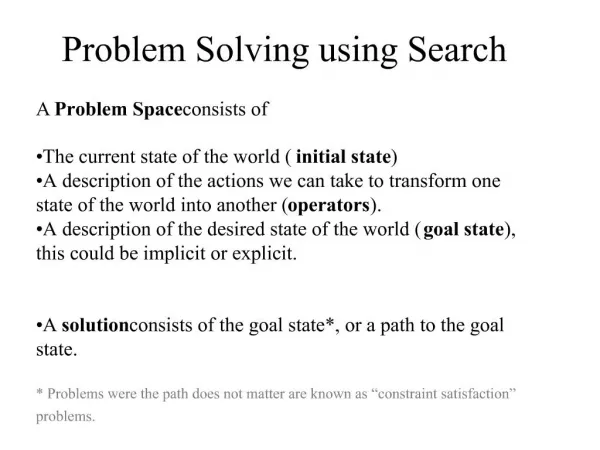
Defining and Representing the Problem • State space: The combination of the initial state and the set of operators make up the state space of the problem. • Initiate state: The original state of the problem. • Operators: used to modify the current state, thereby creating a new state. • Path: The sequence of states produced by the valid application of operators from an old state to a new state is called the path. • Goal state: A state fit to the searching objective is called the goal state.
Descriptions of Problem Solving • In many search problem, we are not only interested in reaching a go al state, we would like to reach it with the lowest cost (or the maximum profit). • We can compute a cost as we apply operators and transit from state to state. • The path cost or cost function is usually denoted by g. • Given a problem which can be represented by a set os states and operators and then solves using a search algorithm. • For many real-world problems the search space can grow very large, so we need algorithms to deal with that.
Descriptions of Problem Solving • Effective search algorithm must do two things: cause motion or traversal of the state space, and do so in a controlled or systematic manner. • The method that never using the information about the problem to help direct the search is called brute-force, uninformed, or blind search. • Search algorithms which use information about the problem, such as the cost or distance to the goal state, are called heuristic, informed, or directed search.
Descriptions of Problem Solving • An algorithm is optimal if it will find the best solution from among several possible solutions. • A strategy is complete if it guarantees that it will find a solution if one exists. • The complexity of the algorithm , in terms of time complexity (how long it takes to find a solution) and space complexity (how much memory it require), is a major practical considerations. • In real-world, the search problem can be classified to two classes: P and NP.
Descriptions of Problem Solving • In real-world, the search problem can be classified to two classes: P and NP. • The classes P consists of all problems for which algorithms with polynomial time behavior have been found. • The class NP is essentially the set of problems for which algorithms with exponential behavior have been found. • If an optimization of the problem cannot be solved in polynomial time, it is called NP-hard.
Common Problem Solving Methods • 線性規劃法 (Linear Programming: LP) • 整數規劃法 (Integer Programming) • 分支界限法 (Branch and Bound Method) • 啟發式解法:MST, RMST, SA • Kruskal, 1956; Prim, 1959; Dijkstra, 1959; Sollin, 1965; Yu, 1998 • 全域搜尋法 (Global Searching):GA • Brute-Force Search Method
Brute Force Search Techniques • Breadth-First Search (BFS) • Depth-First Search (DFS)
Algorithm of Breadth-First Search • Create the queue and add the first Node to it. • Loop: • If the queue is empty, quit. • Remove the first Node from the queue. • If the Node contains the goal state, then exit with the Node as the solution. • For each child of the current Node: Add the new state to the back of the queue.
Algorithm of Depth-First Search • Create the queue and add the first SearchNode to it. • Loop: • If the queue is empty, quit. • Remove the first SearchNode from the queue. • If the Node contains the goal state, then exit with the SearchNode as the solution. • For each child of the current SearchNode : Add the new state to the front of the queue.
汶水 獅潭 三灣 新竹 公館 頭份 頭屋 尖山 竹南 造橋 苗栗 後龍 Example從苗栗到新竹之可能路徑
The path generated by BFS [苗栗] ←[苗栗], [公館][頭屋][造橋][後龍] ← [公館], [頭屋][造橋][後龍][汶水] ← [頭屋], [造橋][後龍][汶水][尖山] ← [造橋], [後龍][汶水][尖山] ← [後龍], [汶水][尖山] ← [汶水], [尖山][獅潭] ← [尖山], [獅潭][頭份][竹南] ← [獅潭], [頭份][竹南][三灣] ← [頭份], [竹南][三灣][新竹] ← [竹南], [三灣][新竹] ← [三灣], [新竹] ← [新竹]
The path generated by DFS [苗栗] ←[苗栗], [後龍][造橋][頭屋][公館] ←[後龍], [尖山][造橋][頭屋][公館] ←[尖山], [竹南][頭份][造橋][頭屋][公館] ←[竹南], [新竹][頭份][造橋][頭屋][公館] ←[新竹], [頭份][造橋][頭屋][公館]
Improving DFS The DFS algorithm can be improved by adding a parameter to limit the search to a maximum depth of the tree. Then we add a control loop where we continuously deepen our DFS until we find the solution.
TSP Problem Definition The Traveling Salesman Problem (TSP), where a salesman makes a complete tour of the cities on his route, visiting each city exactly once, while traveling the shortest possible distance, is an example of a problem which has a combinatorial explosion. As such, it cannot be solved using BFS or DFS for problems of any realistic size. TSP belongs to a class of problems known as NP-hard or NP-complete.
Searching method for TSP Problem Finding the best possible answer is not computationally feasible, and so we have to settle a good answer. Several heuristic search methods are employed to solve this type of problem. • Generate and Test (GAT) • Best-First Search (BFS) • Greedy Search (GS) • A* Search • Constraint Satisfaction (CS) • Mean-Ends Analysis (MEA)
The Algorithm of GAT • Generate a possible solution, either a new state or a path through the problem space. • Test to see if the new state or path is a solution by comparing it to a set of goal states. • If a solution has been found, return success; else return to step 1.
The modification of GAT To avoid getting trapped in a suboptimal states, variations on the hill climbing strategy have been proposed. One is to inject noise into the evaluation function, with the initial noise level high and slowly decreasingly over time. This technique, called simulated annealing, allows the search algorithm to go in directions which are not “best” but allow more complete exploration of the search space. (Kirkpartrick, Gelatt, and Vecchi, 1983)
The Algorithm of BFS BFS is a systematic control strategy, combining the strengths of breadth-first and depth-first search into one algorithm. The main difference between BFS and the brute-force search techniques is that we make use of an evaluation or heuristic function to order the SearchNode objects on the queue. In this way, we choose the SearchNode that appears to be best, before any others, regardless of their position in the tree or graph.
The Algorithm of Greedy Search GS is a best-first strategy where we try to minimize the estimated cost to reach the goal. Since we are greedy, we always expand the node that is estimated to be closest to the goal state. Unfortunately, the exact cost of reaching the goal state usually can’t be computed, but we can estimate it by using a cost estimate or heuristic function h().
A* Search One of the famous search algorithms used in AI is A* search algorithm, which combines the greedy algorithm for efficiency with the uniform-cost search for optimality and completeness. In A* the evaluation function is computed by adding the two heuristic measures; the h(n) cost estimate of traveling from n to the goal state, and g(n) which is the known path cost from the start node to n into a function called f(n).
The Algorithm of Constraint Satisfaction Usually, all problems have some constraints which define what the acceptable solutions are. For example, if our problem is to load a delivery truck with packages, a constraint may be that the truck holds only 2000 pounds. This constraint could help us substantially reduce our search space by ignoring search paths uses a set of constraints to define the space of acceptable solutions.
Means-Ends Analysis MEA is a process for problem solving which is based on detecting differences between states and then trying to reduce those differences. First used in the General Problem Solver (Newell and Simon, 1963), MEA uses both forward and backward reasoning and a recursive algorithm to systematically minimize the differences between the initial and the goal states.
The Algorithm of MEA • Compare the current-state to the goal-state. If states are identical then return success. • Select the most important difference and reduce it by performing the following steps until success or failure: • Select an operator that is applicable to the current difference. If there are no operators which can be applied, then return failure. • Attempt to apply the operator to the current state by generating two temporary states, one where the operator’s preconditions are true (prestate), and one that would be the result if the operator were applied to the current state (poststate).
The Algorithm of MEA iii. Divide the problem into two parts, a First part, from the current state to the prestate, and a Last part, from the poststate to the goal state. Call MEA to solve both pieces. If both are true, then return success, with the solution consisting of the First part, the selected operator, and the Last part.