Basic Problem Solving Search strategy
This document explores the fundamental concepts of problem-solving through state space search. It describes transforming an initial state into a goal state by navigating intermediate states. Two primary search methods are detailed: forward reasoning, which goes from the initial state to the goal, and backward reasoning, which starts at the goal and works back to find the initial state. It also discusses systematic uninformed search strategies like Breadth-First Search (BFS) and Depth-First Search (DFS), highlighting their mechanisms, advantages, and algorithmic implementations.

Basic Problem Solving Search strategy
E N D
Presentation Transcript
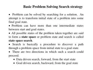
Basic Problem Solving Search strategy • Problem can be solved by searching for a solution. An attempt is to transform initial state of a problem into some final goal state. • Problem can have more than one intermediate states between start and goal states. • All possible states of the problem taken together are said to form a state space or problem state and search is called state space search. • Search is basically a procedure to discover a path through a problem space from initial state to a goal state. • There are two directions in which such a search could proceed. • Data driven search, forward, from the start state • Goal driven search, backward, from the goal state
Forward Reasoning (Chaining): Control strategy that starts with known facts and works towards a conclusion. • - For example in 8 puzzle problem, we start from initial state to goal state. • In this case we begin building a tree of move sequences with initial state as the root of the tree. • Generate the next level of the tree by finding all rules whose left sides match with root and use their right side to create the new state. • Continue until a configuration that matches the goal state is generated. • Language OPS5 uses forward reasoning rules. Rules are expressed in the form of “if-then rule”. Find out sub-goals which could generate the given goal.
Backward reasoning (Chaining): It is a goal directed control strategy that begins with the final goal. Continue to work backward, generating more sub goals that must also be satisfied until all the sub goals have been met. Prolog (Programming in Logic) uses this strategy. Remark1: In 8 puzzle problem with a single initial state and a single goal state, it makes no difference whether the problem is solved in the forward or the backward direction. The computational effort is the same. In both these cases, same state space is searched but in different order. Remark2: If there are large number of explicit goal states and one initial state, then it would not be efficient to try to solve this in backward direction because we don’t know which goal state is closest to the initial state. So it is better to reason forward.
General observations • Move from the smaller set of states to the larger set of states. • Proceed in the direction with the lower branching factor (the average number of nodes that can be reached directly from single node) • Example: In mathematics, suppose we have to prove a theorem. There are initial states as small set of axioms. • From these set of axioms, we can drive a very large number of theorems. • On the other hand, the large number of theorems must go back to the small set of axioms. So branching factor is significantly greater going forward from axioms to theorem than it is going from theorems to axioms.
General Purpose Search Strategies • Let us discuss some of systematic uninformed searches. • 1. Breadth First Search (BFS) • It expands all the states one step away from the initial state, then expands all states two steps from initial state, then three steps etc., until a goal state is reached. • That is, it expands all nodes at a given depth before expanding any nodes at a greater depth. • So All nodes at the same level are searched before going to the next level down. • We can implement it by using two lists called OPEN and CLOSED. The OPEN list contains those states that are to be expanded and CLOSED list keeps track of states already expanded. Here OPEN list is used as a queue.
Algorithm (BFS) • Input: Two states in the state space START and GOAL • Local Variables: OPEN, CLOSED, STATE-X, SUCCS • Output: Yes or No • Method: • Initially OPEN list contains a START node and CLOSED list is empty; Found = false; • While (OPEN empty and Found = false) • Do { • Remove the first state from OPEN and call it STATE-X; • Put STATE-X in the front of CLOSED list; • If STATE-X = GOAL then Found = true else • {- perform EXPAND operation on STATE-X, producing a list of SUCCESSORS; • - Remove from successors those states, if any, that are in the CLOSED list; • - Append SUCCESSORS at the end of the OPEN list /*queue*/ • } } /* end while */ • If Found = true then return Yes else return No and Stop
2. Depth - first search : • In depth-first search we go as far down as possible into the search tree / graph before backing up and trying alternatives. • It works by always generating a descendent of the most recently expanded node until some depth cut off is reached and then backtracks to next most recently expanded node and generates one of its descendants. • So only path of nodes from the initial node to the current node is stored in order to execute the algorithm. • It avoids memory limitation as it only stores a single path from the root to leaf node along with the remaining unexpanded siblings for each node on the path.
We will again use two lists called OPEN and CLOSED with the same conventions explained earlier. Here OPEN list is used as a stack • If we discover that first element of OPEN is the Goal state, then search terminates successfully. • We could get track of our path through state space as we traversed but in those situations where many nodes after expansion are in the closed list, then we fail to keep track of our path. • This information can be obtained by modifying CLOSED list by putting pointer back to its parent in the search tree.
Algorithms (DFS) • Input: Two states in the state space, START and GOAL • LOCAL Variables: OPEN, CLOSED, RECORD-X, SUCCESSORS • Output: A path sequence if one exists, otherwise return No • Method: • Form a queue consisting of (START, nil) and call it OPEN list. Initially set CLOSED list as empty; Found = false; • While (OPEN empty and Found = false) DO • { • Remove the first state from OPEN and call it RECORD-X; • Put RECORD-X in the front of CLOSED list; • If the state variable of RECORD-X= GOAL, • then Found = true
Else • { - Perform EXPAND operation on STATE-X, a state variable of RECORD-X, producing a list of action records called SUCCESSORS; create each action record by associating with each state its parent. • - Remove from SUCCESSORS any record whose state variables are in the record already in the CLOSED list. • - Insert SUCCESSORS in the front of the OPEN list /* Stack */ • } • }/* end while */ • If Found = true then return the plan used /* find it by tracing through the pointers on the CLOSED list */ else return No • Stop
Comparisons: (These are unguided / blind searches, we can not say much about them) • DFS is effective when there are few sub trees in the search tree that have only one connection point to the rest of the states. • DFS can be dangerous when the path closer to the START and farther from the GOAL has been chosen. • DFS is best when the GOAL exists in the lower left portion of the search tree. • BFS is effective when the search tree has a low branching factor. • BFS can work even in trees that are infinitely deep. • BFS requires a lot of memory as number of nodes in level of the tree increases exponentially. • BFS is superior when the GOAL exists in the upper right portion of a search tree.
3. Depth First Iterative Deepening (DFID) : • An optimal Admissible Tree search, by Richard G. Korf, Artificial Intelligence 27(1985) pp 97-109 • . It suffers neither the drawbacks of BFS nor of DFS on trees • It takes advantages of both the strategies. • Since DFID expands all nodes at a given depth before expanding any nodes at greater depth, it is guaranteed to find a shortest - length (path) solution from initial state to goal state.
Algorithm (DFID) • Initialize d = 1 /* depth of search tree */ , Found = false • While (Found = false) • DO { - perform a depth first search from start to depth d. - if goal state is obtained then Found = true else discarding the nodes generated in the search of depth d - d = d + 1 • }/* end while */ • Report the solution • Stop
At any given time, it is performing a DFS and never searches deeper than depth d the space it uses is O(d). • Disadvantage of DFID is that it performs wasted computation prior to reaching the goal depth. • Analysis of Search methods • Effectiveness of a search strategy in problem solving can be measured in terms of: • Completeness: Does it guarantees a solution when there is one? • Time Complexity: How long does it take to find a solution? • Space Complexity: How much space does it needs? • Optimality: Does it find the highest quality solution when there are several different solutions for the problem?
1. BFS • In worst case BFS must generate all nodes up to depth d • 1 + b + b2 +b3 + …+ bd = O(bd) • Note on average, half of the nodes at depth d must be examined and so average case time complexity is O(bd) • Space complexity - O(bd) 2. DFS • If the depth cut off is d the space requirement is O(d) • In worst, the time complexity of DFS to depth d = O(bd) • DFS requires an arbitrary cut off depth. If branches are not cut off and duplicates are not checked for, the algorithm may not terminate.
3. DFID • Time requirement for DFID on tree • nodes at depth d are generated once during the final iteration of the search • nodes at depth d-1 are generated twice • nodes at depth d-2 are generated thrice and so on. • Thus the total number of nodes generated in DFID to depth d are • T = bd + 2bd-1 + 3bd-2 + …. db • = bd [1 + 2b-1 + 3b-2 + ….db1-d] • = bd [1 + 2x +3x2 + 4x3 + …. • + dxd-1] { if x = b-1} • T converges to bd (1-x)-2 for | x | < 1. Since (1-x)-2 is a constant and independent of d, if b > 1, T O(bd)
Time Space Solution • BFS O(bd) O(bd) Optimal • DFS O(bd) O(d) ---- • DFID O(bd) O(d) Optimal
4. Bi-directional Search • For those problems having a single goal state and single start state, bi-directional search can be used. • It starts searching forward from initial state and backward from the goal state simultaneously starting the states generated until a common state is found on both search frontiers. • DFID can be applied to bi-directional search as follows for k = 1, 2, ..: • kth iteration consists of a DFS from one direction to depth k storing only the states at depth k, and DFS from other direction : one to depth k and other to depth k+1 not storing states but simply matching against the stored states from other direction. / * The search to depth k+1 is necessary to find odd-length solutions */.
Graph: • Start • 1 • 2 3 4 • 5 6 7 8 9 • 10 11 12 13 • 14 15 • 16 • Goal
For k = 0 Start • 1 • ______________ • 14 15 • 16 • Goal
For k = 1 • Start • 1 • 2 3 4 • _________________________________ • 11 12 13 • 14 15 • 16 • Goal
For k = 2 • Start • 1 • 2 3 4 • 5 6 7 8 9 • _____________________________________________ • 11 • 14 • 16 • Goal