Using Search in Problem Solving
This guide provides an overview of search methods in problem-solving, focusing on search spaces, trees, and graphs. It explains how search problems can be modeled as graphs where nodes represent states and edges represent operations to transition between states. Key search techniques such as uninformed (depth-first and breadth-first) and informed search methods (A*, hill climbing) are discussed. Additionally, the differences between various search algorithms, their advantages, and how they navigate through the search space to find optimal paths are explored, offering valuable insights for both theoretical and practical applications in AI.

Using Search in Problem Solving
E N D
Presentation Transcript
Search and AI • Introduction • Search Space, Search Trees • Search in Graphs • Search Methods • Uninformed search • Breadth-first • Depth-first
Introduction • you know the available actions that you could perform to solve your problem • you don't know which ones in particular should be used and in what sequence, in order to obtain a solution • you can search through all the possibilities to find one particular sequence of actions that will give a solution.
The Scenario Initialstate Target (Goal) state A set of intermediate states A set of operations, that move us from one state to another. The task:Find a sequence of operations that will move us from the initial state to the target state. Solved in terms of searching a graph The set of all states: search space
Initial state Target state
Search Space • Search problems can be represented as graphs, where the nodes are states and the arcs correspond to operations. • The set of all states: search space
Graphs and Trees 1 • Graph: a set of nodes (vertices) with links(edges) between them. A link is represented usually as a pair of nodes, connected by the link. • Undirected graphs: the links do not have orientation • Directed graphs: the links have orientation
Graphs and Trees 2 • Path:Sequence of nodes such that each two neighbors represent an edge • Cycle: a path with the first node equal to the last and no other nodes are repeated • Acyclic graph: a graph without cycles • Tree: undirected acyclic graph, where one node is chosen to be the root
Graphs and Trees 3 • Given a graph and a node: • Out-going edges:all edges that start in that node • In-coming edges :all edges that end up in that node • Successors (Children):the end nodes of all out-going edges • Ancestors (Parents):the nodes that are start points of in-coming edges
G1: Undirected graph A B C D E Path: ABDCAE Cycle: CABEC Successors of A: E, C, B Parents of A: E, C, B
A B G2: Directed graph C D E Path: ABDC Cycle: no cycles Successors of A: C, B Parent of A: E
Search Trees • More solutions: More than one path from the initial state to a goal state • Different paths may have common arcs • The search process can be represented by a search tree • In the search tree the different solutions will be represented as different paths from the initial state • One and the same state may be represented by different nodes
Search Methods • Uninformed (blind, exhaustive) search • Depth-first • Breadth-first • Informed (heuristic) search • Hill climbing • Best-first search • A* search
Exhaustive Search • Breadth-first • Depth-First • Iterative Deepening
Breadth-First Search Algorithm: using a queue 1. Queue = [initial_node] , FOUND = False 2. While queue not empty and FOUND = False do: Remove the first node N If N = target node then FOUND = true Elsefind all successor nodes of N and put them into the queue. In essence this is Dijkstra's algorithm of finding the shortest path between two nodes in a graph.
Depth-first search Algorithm: using a stack 1. Stack = [initial_node] , FOUND = False 2. While stack not empty and FOUND = False do: Remove the top node N If N = target node then FOUND = true Else find all successor nodes of N and put them onto the stack.
Depth-First Iterative Deepening • An exhaustive search method based on both depth-first and breadth-first search. • Carries out depth-first search to depth of 1, then to depth of 2, 3, and so on until a goal node is found. • Efficient in memory use, and can cope with infinitely long branches. • Not as inefficient in time as it might appear, particularly for very large trees, in which it only needs to examine the largest row (the last one) once.
Comparison of depth-first and breadth-first search Breadth-first: without backtracking Depth-first : backtracking. Length of path:breadth-first finds the shortest path first. Memory:depth-first uses less memory Time:If the solution is on a short path - breadth first is better, if the path is long - depth first is better.
The Search Space • The search space is known in advance e.g. finding a map route • The search space is created while solving the problem - e.g. game playing
Generate and Test Approach Search tree - built during the search process Root- corresponds to the initial state Nodes: correspond to intermediate states (two different nodes may correspond to one and the same state) Links- correspond to the operators applied to move from one state to the next state Node description
Node Description • The corresponding state • The parent node • The operator applied • The length of the path from the root to that node • The cost of the path
Node Generation • To expand a node means to apply operators to the node and obtain next nodes in the tree i.e. to generate its successors. • Successor nodes: obtained from the current node by applying the operators
Algorithm • Store root (initial state) in stack/queue • While there are nodes in stack/queue DO: • Take a node • While there are applicable operators DO: • Generate next state/node (by an operator) • If goal state is reached - stop • If the state is not repeated - add into stack/queue • To get the solution: Print the path from the root to the found goal state
Example - the Jugs problem • We have to decide: • representation of the problem state, initial and final states • representation of the actions available in the problem, in terms of how they change the problem state. • what would be the cost of the solution • Path cost • Search cost
Problem representation • Problem state: a pair of numbers (X,Y): • X - water in jar 1 called A, • Y - water in jar 2, called B. • Initial state: (0,0) • Final state: (2, _ ) • here "_" means "any quantity"
Operations for the Jugs problem Operators: Preconditions Effects O1. Fill A X < 4 (4, Y) O2. Fill B Y < 3 (X, 3) O3. Empty A X > 0 (0, Y) O4. Empty B Y > 0 (X, 0) O5. Pour A into B X > 3 - Y ( X + Y - 3 , 3) X 3 - Y ( 0, X + Y) O6. Pour B into A Y > 4 - X (4, X + Y - 4) Y 4 - X ( X + Y, 0)
0,0 O1 O2 3,0 0,4 O2 O6 O5 O1 3,4 0,3 3,4 3,1 Search tree built in a breadth-first manner
The A* Algorithm A* always finds the best solution, provided that h(Node) does not overestimate the future costs.
A 4 10 2 9 H : 5 B: 9 D : 10 4 F : 6 2 4 6 C: 8 K: 5 E: 7 8 10 7 8 J: 4 G: 0 Example Start: A Goal: G