Classical Electromagnetism ie, advanced electromagnetism

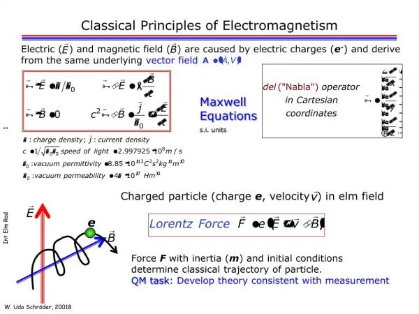
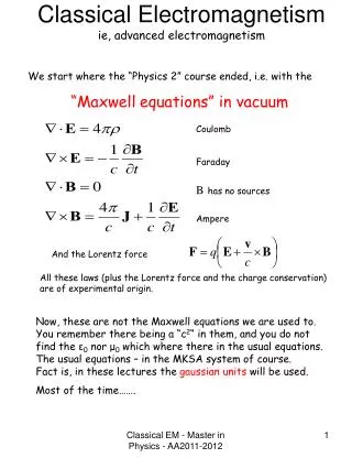
1. We start where the “Physics 2” course ended, i.e. with the “Maxwellequations” in vacuum Coulomb Faraday Classical Electromagnetismie, advanced electromagnetism Bhas no sources Ampere And the Lorentz force All these laws (plus the Lorentz force and the charge conservation) are of experimental origin. Now, these are not the Maxwell equations we are used to. You remember there being a “c2“ in them, and you do not find the ε0 nor μ0 which where there in the usual equations. The usual equations – in the MKSA system of course. Fact is, in these lectures the gaussian units will be used. Most of the time……. Classical EM - Master in Physics - AA2011-2012

2. The Maxwell equations in vacuum in the SI system have the following, familiar, form: Gauss’s law Faraday’s law No magnetic monopoles Ampere’s law With the usual addition of the Lorentz’s force: In the Gaussian units the units of charge are not defined experimentally, but are derived from the Coulomb’s law The magnetic quantities are defined by writing the law of Biot-Savart as Where the mechanical units are measured in the cgs system. Classical EM - Master in Physics - AA2011-2012

3. Why a new system of units? Because the one widely in use across the earth (MKSA) is practical to use in technical activities, but from a “theoretical” point of view (including in the word also the better understanding of the physical phenomena), has useless and also misleading consequences. E and B seem in MKSA to be two completely independent quantities, but in Gaussian units they have the same dimensions and turn eventually out to be different components of the same quantity. Also important is to have taken away from the equations the two quantities and and replaced them with the much more meaningful “c”. A slightly modified form of the Gaussian system exists, and is in use in the book by Mel Schwartz. It is called modified Gauss, and the modification consists of writing Instead of Classical EM - Master in Physics - AA2011-2012

4. Electrostatics Electrostatics and Magnetostatics have been treated in depth in the previous courses, and we assume that the conservative nature of electrostatic force, the existence and basic properties of the electrostatic potential, the principle of superposition, the conservation of charge, are well known. We already know then that, given a charge distribution ρ in space the electric field is computed from the potential with the formula And the potential is the solution of the equations To solve for the field with this formula we need to know the charge distribution ρ. Many problems can be amenable to this one, but many are not: just think of those in which the boundary conditions are the potentials at the surface of some conductors. To solve this type of problems (Dirichlet problems) we need another approach. Classical EM - Master in Physics - AA2011-2012

5. The ψ angle is chosen around the axis of symmetry of the system. The condition of symmetry around that axis is mathematically expressed as independence of potential and charge distributions from ψ. To solve the Laplace or Poisson equations we first need to express the laplacian in spherical coordinates. We know the formula for the laplacian in cartesian coordinates. We could then express the cartesian coordinates as function of the spherical ones and compute the laplacian via this dependence as a function of the spherical ones. With the help of a few sheets of paper we can do that. We shall instead use two formulas: To show how to proceed in such cases let us study a simple case: a configuration of potential which has an axial symmetry, i.e. a symmetry for rotations about an axis. In such cases it is convenient to use the spherical coordinates (r,θ,ψ), and: Ie, the laplacian of a function of space is the divergence of its gradient. And, the Gauss’s theorem: ie, the infinitesimal flux of any vector P through an infinitesimal volume element dV is equal to the divergence of Ptimes dV. What we have to do now is to replace P with the gradient of Φ. Classical EM - Master in Physics - AA2011-2012

6. Classical EM - Master in Physics - AA2011-2012

7. Let us now replace the generic vectorA with the gradΦ: We get then the part of the flux of A which flows through the infinitesimal surfaces 1 and 2 of the infinitesimal volume dV: The other 2 components can be calculated (if you really want to….) in the same way; by adding all three the formula for the laplacian is obtained. Classical EM - Master in Physics - AA2011-2012

8. We start the search of a solution in the region where there are NO Charges. There the Laplace equation holds Since we study the case of symmetry, And the equation loses its last term. Still, it is complicated by the too many sinθ, so we apply a change of variables And our Laplace equation becomes We will search now NOT the right solution (a differential equation usually has an infinite number of solutions), but SIMPLE solutions. In this case, simple stands for factorizable, ie: And the Laplace equation becomes (next page) Classical EM - Master in Physics - AA2011-2012

9. The function on the left side is a function only of r, while that on the right is a function only of μ. If they are to be equal over the whole range of r andμthey must be independent of both r andμand therefore be a constant, which we call K. We still have not found a solution, so let’s look for a SIMPLE one for F(r): a series of powers in r. With the condition that F may diverge only at r = 0 (point charge at the origin) or at infinity (constant field). The equation for F(r) then becomes: With n entire, positive or negative. n being entire, only some (entire) values are allowed for K = n(n+1)) Classical EM - Master in Physics - AA2011-2012

10. And the Φ(r,θ) becomes: Now we must find – for each n- the corresponding Pnby solving its differential equation with its K=n(n+1): Having before had so much success with the radial function F we try a power series also for theμdependence Pn(μ) = ΣAn,lμl The differential equationbecomes l=0,∞ It has a solution IF: This is a recurrence relation which allows to compute all terms with l even (all terms with l odd) once we know An,0 (An,1). Let us start with n even. All terms with l even larger than n will be zero. The same will happen to the l odd terms with n odd. Classical EM - Master in Physics - AA2011-2012

11. So far we have seen that the recursive relation has the effect to limit the number of elements of the series for and n being both even or both odd. But the recursive relation has no effect on the elements with land n one even and the other odd. In fact, the high values of ltend to a constant value and the series would diverge. The only way to have a reasonable (i.e., not-infinite) result is to set equal to zero all coefficients An,l of different “parity”: For n even, all terms with l odd are null. For n odd, all terms with l even are null. At this point, we know that there are many radial functions, depending on the values of K, and therefore on n. To each of these is associated a function Pnot μ and therefore of θwhich is the sum of n/2 terms: all terms are defined apart from a common factor, which is defined by imposing the “normalization” condition The Pn are called – as you probably have already guessed - Legendre polynomials. The first 4 are listed below: Classical EM - Master in Physics - AA2011-2012

12. And eventually the potential becomes: This formula is the expression of the electrostatic potential as a series of multipoles. Monopole, dipole, quadrupole, octupole etc. Remember, this development is possible only in the caseof systems with symmetry around an axis. Note that only a single multipole is a factorized function. A generic potential which is the sum of at least 2 different multipoles is NOT factorizable. The problem of determining the potential – with given boundary conditions, of course – is reduced to the problem of the determination of the coefficients.The Legendre polynomials Pn(cosθ) are a COMPLETE AND ORTHOGONAL SYSTEM of functions in the interval -1 ≤ μ≤ 1. The orthogonality of the polynomials is expressed by the formula: Given an arbitrary regular function f(μ) in the given range, it can be written as Where the coefficients Anare computed using the orthogonality condition. Classical EM - Master in Physics - AA2011-2012

13. Examples • A sphere with radius R. On its surface the potential Φ(R,θ) is known. There are no other charges. The potential at large distances is 0. The condition that the potential goes to 0 at large distances requires that all An’sare equal to zero –outside the sphere. The condition that inside the sphere there are no charges requires that the potential be finite inside, in particular for r=0. This condition requires that all Bn be equal to zero inside the sphere. Therefore : Inside the sphere Outside the sphere The two regions – inside and outside the sphere – are treated separately with two different distributions because they are two different regions without charges. At the sphere surface, the two potentials must take the value which is given in the problem as a boundary condition: where the coefficients Anand Bnare computed at the sphere surface: Classical EM - Master in Physics - AA2011-2012

14. where the coefficients Anand Bnare computed at the sphere surface: The continuity of the potential at the sphere surface is the condition that has been imposed to compute the coefficients. Note that the coefficients for both potentials –inside and outside – have been computed with the same integral in and are therefore correlated. It turns out that: And therefore 2) A sphere (radius R) at a constant potential Φ0. We know already that the potential inside is constant (Φ0), while outside it has a Φ0R/r behaviour. Let us find it out with our formulas. Classical EM - Master in Physics - AA2011-2012

15. And, as a consequence, the potential is 3rd Exercise: a conducting “small” sphere at ground voltage (“zero” potential ) placed in a “large” constant field. The insertion of the ball will modify the field around it. But the “small” and the “large” specifications indicate that we can approximate the field at “large” distances from it as a uniform field, let us choose the reference system with the axis of symmetry passing the sphere center and directed parallel to the uniform field. At large distances from the ball the field will be directed along, say, the “z” axis and the potential will be of the type The field turns out to be a dipole. Which, of course, can go on for large distances compare to the ball’s size, but obviously not forever. The ball itself is however at zero potential. Since the only non-zero term in the series is the dipole (n=1), then: Evaluating this formula at the sphere radius r = R and setting itto 0 we find that B1 = E0R3and the potential is Classical EM - Master in Physics - AA2011-2012

16. Last remark before going on: the condition we required at the beginning to deal only with azimuthally symmetric system is not necessary: the consequence of that condition is that we end up with the Legendre polynomials, which have a rather simple expression. If we deal with ”any” system, not symmetric, we will end up with more complicated angular functions (associated Legendre functions and spherical harmonics, Jackson 3.5). Recapitulate Note that an azimuthal symmetry does not necessarily mean a sphere. It could be a bottle (not a Coca Cola bottle), a lampshade, a pear,….. These are all cases of symmetry in ψ but not in . We have found a general solution for the potential in a region free of charges for cases in which the boundary condition is given as the potential function on the boundaries of the charge free region, and is, of course, azimuthally symmetric. This general solution is called expansion in series of multipoles and takes the form of where the coefficients An andBn are determined by requiring the series to satisfy the boundary condition. The polynomials Pn are functions of cosθ odd or even according to n. The radial dependence of the potential is a (sum of two) powers of r, of which one describes the potential Outside the boundary surface and the other Inside. Note that the r dependence, which used to be of the type 1/r,for a multipole of order n becomes 1/rn+1for large r. Classical EM - Master in Physics - AA2011-2012

17. Note that each Pn has exactly n zeros in the range of -1≤cosθ≤1 Classical EM - Master in Physics - AA2011-2012

18. Multipole expansion of the potential from a charge distribution with azimuthal symmetry Now consider the case in which the boundary condition is not given as the potential over a surface but as charge distributions in space (always with azimuthal symmetry). But… in such case a solution exists, yes, and.. We already know it. Why bother to try and find a different one? The solution we already know is: This is the general solution. Very general…. We still want to express the solution in the form of a multipole expansion: because there is a lot of physical meaning in it. We know what a multipole has for an angular dependence, and also for a radial dependence. The multipole expansion is valid in a region without charges. Well, given such a region, there are two cases, which we will distinguish: The charges are at smaller radius than the point where want to determine the potential; and The charges are at larger radius. Ie, internal and external charges. Of course, the superposition principle will aid in the determination of the potential in the general case. Classical EM - Master in Physics - AA2011-2012

19. We start with the case of internal charge distribution . The solution will have the form: Now what we need is to expand in series of r the general formula We expand in power series a function of type to obtain We now have to integrate over ψ and ψ’, taking advantage of the fact that ρ does not depend on ψ. The only thing that varies in the integral is the product . Therefore we can set ψ=0 (because of the symmetry of the charge distribution and average over ψ’. Classical EM - Master in Physics - AA2011-2012

20. We are now in a position to calculate the powers of averaged over ψ’. And eventually Which leads us to: And, in a concentrated formula Comparing this formula with the previous general one we expected to get: We finally obtain the formula for the coefficients Bn which are computed from the charge distribution ρ. Classical EM - Master in Physics - AA2011-2012

21. +q +q 2d -q +q What have we obtained now? We have expanded a charge distribution constrained only to be azimuthally symmetric into a multipole series. This not only a mathematical game: now we can speak of a charge distribution having a dipole moment (already known….), quadrupole moment, mainly this or mainly that. And we will know with which power of r will the potential decay at large distances. Let us compute the first moments and see what they look like. Total charge Dipole moment (remember?) Quadrupole moment B0 = +q-q = 0 Monopole B1 = qd +(-q)(-d) = 2qd Dipole B2 = qd2 + (-q)d2 = 0 Quadrupole B0 = +q-2q+q = 0 Monopole B1 = qd +2q*0+(+q)(-d) = 0 Dipole B2 = qd2+(-2q)*(0)+(+q)d2 = 2qd2 Quadrupole 2d -2q Classical EM - Master in Physics - AA2011-2012

22. What has been obtained so far is the potential in a charge free region, generated by a charge distribution inside the potential region. What we can do now is solve the inverse problem: given a hollow charge distribution, how can we calculate the potential in the charge-free region inside it? The problem is mathematically equal to the previous one, with the only inversion of r and r’. The result will be very similar: Where the coefficients An, the multipole moments of the charge distribution are given by the formula: The two multipole expansions – for charge distributions inside and outside the sphere on whose surface lies the point where we want to know the potential- can be added to compute the potential in every point in space, even within the charge distribution. Classical EM - Master in Physics - AA2011-2012

23. Electrostatic Energy The Electrostatic Energy of a charge distribution ρis given by the formula: This formula is simply the generalization of the formula for the energy of the system of two charges: It tells us that the electrostatic energy is distributed in space and is non-zero only where charges are present! The integral is in fact equal to zero where ρ=0. We have before developed a formula which gives us the potential in all situations in which charges are present both inside and outside the point where we compute. We can even imagine a system in which two azimuthally symmetric charge distributions are at work, one inside the other; and they are separated by a more or less large charge-free region. (Btw, could you find in nature an example of such a system?) Let us examine this case, and call the two charge distributions ρ1andρ2. They will give origin in the free space in between to the potentials Φ1andΦ2, and the total potential there will be Φ = Φ1 + Φ2. The total electrostatic energy: Classical EM - Master in Physics - AA2011-2012

24. Self energies of the two charge distributions Interaction energies Let us compute a term of the interaction energy: The two interaction energies are equal!!! And now, for a system which has azimutal symmetry and therefore has charge density and potential parametrizable as series of Legendre polynomials: The substitution of the 2 indices “1” And “2” with the indices “e” and “n” for the two charge distribution is NOT casual. Classical EM - Master in Physics - AA2011-2012

25. The density distribution of the electron cloud in atoms is usually very well known. This knowledge allows for each atom a precise determination of its multipole moments – in particular of its quadrupole moments. An accurate measurement of the interaction energy of the two charges allows a determination of the quadrupole moment of the nucleus –or at least of its sign – which indicates at the very least if the nucleus has a non-spherical shape; and which way it is non-spherical. Being it a symmetrical system around one axis, it can be cigar-like (egg-like) or pancake-like. The nucleus charge distribution being all positive, a positive moment will indicate a cigar-like shape. Classical EM - Master in Physics - AA2011-2012

26. Classical EM - Master in Physics - AA2011-2012