Download
1 / 31
310 likes | 499 Vues
Flow and Energy Momentum Tensor From Classical Gluon Fields. Rainer J. Fries Texas A&M University. NFQCD Kyoto, December 5 , 2013. Overview. Classical Gluon Fields and MV Model Analytic Solutions for Early Times Phenomenology Beyond Boost-Invariance Work in collaboration mainly with

E N D
Flow and Energy Momentum Tensor From Classical Gluon Fields Rainer J. Fries Texas A&M University NFQCD Kyoto, December 5, 2013
Overview • Classical Gluon Fields and MV Model • Analytic Solutions for Early Times • Phenomenology • Beyond Boost-Invariance Work in collaboration mainly with • Guangyao Chen (Texas A&M) • SenerOzonder (INT/Seattle, Minnesota) NFQCD 2013
The “Standard Model” of URHICs • Bulk evolution • Local thermal equilibrium with small (?) dissipative corrections after time 0.2-1 fm/c. • Expansion and cooling via viscous hydrodynamics. • Hadronic phase: Hydro or Transport. • Pre-equilibrium: color glass condensate (CGC); successful predictions of eccentricities and fluctuations of the energy density flow observables • IP-Glasma • Poor constraints on initial flow and other variables. • p+A? [B. Schenkeet al., PRL108 (2012); C. Gale et al. , PRL 110 (2013)] NFQCD 2013
MV Model: Classical YM Dynamics • Nuclei/hadrons at asymptotically high energy: • Saturated gluon density ~ Qs-2 scale Qs >> QCD, classical fields. • Single nucleus:solve Yang-Mills equations for gluon field A(). • Source = light cone current J (given by SU(3) charge distribution ). • Calculate observables O( ) from the gluon field A(). • fromrandom Gaussian color fluctuations of a color-neutral nucleus. [L. McLerran, R. Venugopalan] NFQCD 2013
MV Model: Classical YM Dynamics • Two nuclei: intersecting currents J1, J2 (given by 1, 2), calculate gluon field A( 1, 2) from YM. • Equations of motion • Boundary conditions [A. Kovner, L. McLerran, H. Weigert] NFQCD 2013
Glasma in the Forward Light Cone • Numerical Solutions of Classical YM in the forward light cone. • Quantum corrections, Instabilities, Thermalization, … • Here: • Analytic solution of classical theory. • Analyze pressure and flow for small times. [Krasnitz, Venugopalan] [T. Lappi] … NFQCD 2013
Fields: Before Collision • Before the collision: color glass = pulse of strictly transverse (color) electric and magnetic fields, mutually orthogonal, with random color orientations, in each nucleus. NFQCD 2013
Fields: At Collision • Before the collision: color glass = pulse of strictly transverse (color) electric and magnetic fields, mutually orthogonal, with random color orientations, in each nucleus. • Immediately after overlap (forward light cone, 0): strong longitudinal electric & magnetic fields. Non-abelian effect. E0 B0 [L. McLerran, T. Lappi, 2006] [RJF, J.I. Kapusta, Y. Li, 2006] NFQCD 2013
Fields: Into the Forward Light Cone • Once the non-abelian longitudinal fields E0, B0 are seeded, the first step of further evolution can be understood in terms of the QCD versions of Ampere’s, Faraday’s and Gauss’ Law. • Longitudinal fields E0, B0 decrease in both z and t away from the light cone • First abeliantheory: • Gauss’ Law at fixed time t • Long. flux imbalance compensated by transverse flux • Gauss: rapidity-odd radialfield • Ampere/Faraday as function of t: • Decreasing long. flux induces transverse field • Ampere/Faraday: rapidity-even curling field • Full classical QCD: [Guangyao Chen, RJF] NFQCD 2013 [G. Chen, RJF, PLB 723 (2013)]
Initial Transverse Field: Visualization • Transverse fields for randomly seeded A1, A2 fields (abelian case). • = 0: Closed field lines around longitudinal flux maxima/minima • 0: Sources/sinks for transverse fields appear NFQCD 2013
Analytic Solution: Small Time Expansion • Here: analytic solution using small-time expansion for gauge field • Recursive solution for gluon field: • 0th order = boundary conditions [RJF, J. Kapusta, Y. Li, 2006] [Fujii, Fukushima, Hidaka, 2009] NFQCD 2013
Analytic Solution: Small Time Expansion • Convergence for weak field limit: recover analytic solution for all times. • Convergence for strong fields: convergence radius ~ 1/Qs for averaged quantities like energy density. NFQCD 2013
Energy Momentum Tensor • Initial ( = 0) structure of the energy-momentum tensor from purely londitudinal fields Transverse pressure PT = 0 Longitudinal pressure PL = –0 NFQCD 2013
Energy Momentum Tensor • Flow emerges from pressure at order 1: • Transverse Poynting vector gives transverse flow. [RJF, J.I. Kapusta, Y. Li, (2006)] [G. Chen, RJF, PLB 723 (2013)] Like hydrodynamic flow, determined by gradient of transverse pressure PT= 0; even in rapidity. Non-hydro like; odd in rapidity ?? NFQCD 2013
Energy Momentum Tensor • Corrections to energy density and pressure due to flow at second order in time • Example: energy density Depletion/increase of energy density due to transverse flow Due to longitudinal flow NFQCD 2013
Transverse Flow: Visualization • Transverse Poynting vector for randomly seeded A1, A2 fields (abelian case). • = 0: “Hydro-like” flow from large to small energy density • 0: Quenching/amplification of flow due to the underlying field structure. NFQCD 2013
Modelling Color Charges • So far color charge densities 1, 2 fixed. • MV: Gaussian distribution around color-neutral average • Sample distribution to obtain event-by-event observables. • Next: analytic calculation of expectation values (as function of average color charge densities 1, 2). • Transverse flow comes from gradients in nuclear profiles. • Original MVmodel = const. • Here: relaxed condition, constant on length scales 1/Qs, allow variations on larger length scales 1/m where m << Qs. [G. Chen, RJF, PLB 723 (2013)] [G. Chen et al., in preparation] NFQCD 2013
Averaged Density and Flow • Energy density ~ product of nuclear gluon distributions ~ product of color source densities • “Hydro” flow: • “Odd“ flow term: • With we have • Order 2 terms … [T. Lappi, 2006] [RJF, Kapusta, Li, 2006] [Fujii, Fukushima, Hidaka, 2009] [G. Chen, RJF, PLB 723 (2013)] [G. Chen et al., in preparation] NFQCD 2013
Higher Orders in Time • Generally: powers of go with factors of Q or factors of transverse gradients • Number of terms with gradients in 1, 2 rises rapidly for higher orders in time. • For the case of near homogeneous charge densities when gradients can be neglected the expressions are fairly simple. • Example: ratio of longitudinal and transverse pressure at midrapidity [G. Chen et al., in preparation] NFQCD 2013
Comparison with Numerical Solutions • Ratio of longitudinal and transverse pressure. Pocket formula for homogeneous nuclei (no transverse gradients): [F. Gelis, T. Epelbaum, arxiv:1307.2214] NFQCD 2013
Comparison with Numerical Solutions • Ratio of longitudinal and transverse pressure. Pocket formula for homogeneous nuclei (no transverse gradients): [F. Gelis, T. Epelbaum, arxiv:1307.2214] NFQCD 2013
Check: Event-By-Event Picture • Example: numerical sampling of charges for “odd” vector i in Au+Au(b=4 fm). • Averaging over events: recover analytic result. Energy density N=1 Analytic expectation value PRELIMINARY NFQCD 2013
Flow Phenomenology: b 0 • Odd flow needs asymmetry between sources. Here: finite impact parameter • Flow field for Au+Au collision, b = 4 fm. • Radial flow following gradients in the fireball at = 0. • In addition: directed flow away from = 0. • Fireball is rotating, exhibits angular momentum. • |V| ~ 0.1 at the surface @ ~ 0.1 NFQCD 2013
Phenomenology: b 0 • Angular momentum is natural: some old models have it, most modern hydro calculations don’t. • Some exceptions • Do we determine flow incorrectly when we miss the rotation? • Directed flow v1: • Compatible with hydro with suitable initial conditions. [L. Csernaiet al. PRC 84 (2011)] … [Gosset, Kapusta, Westfall (1978)] [Liang, Wang (2005)] MV only, integrated over transverse plane, no hydro NFQCD 2013
Phenomenology: A B • Odd flow needs asymmetrybetween sources. Here: asymmetric nuclei. • Flow field for Cu+Au collisions: • Odd flow increases expansion in the wake of the larger nucleus, suppresses flow on the other side. • b0 & A B: non-trivial flow pattern characteristic signatures from classical fields? NFQCD 2013
Phenomenology: A B • CGC fingerprints? Need to evolve systems to larger times. • Examples: Forward-backward asymmetries of type • Here p+Pb: Directed flow asymmetry Radial flow asymmetry NFQCD 2013
Matching to Hydrodynamics • No equilibration here; see other talks at this workshop. • Pragmatic solution: extrapolate from both sides (r() = interpolating fct.) • Here: fast equilibration assumption: • Matching: enforce (and other conservation laws). • Analytic solution possible for matching to ideal hydro. • 4 equations + EOS to determine 5 fields in ideal hydro. Up to second order in time: • Odd flow drops out: we are missing angular momentum! p T L NFQCD 2013
Matching to Hydrodynamics • Instantaneous matching to viscous hydrodynamics using in addition • Mathematically equivalent to imposing smoothness condition on all components of T. • Leads to the same procedure used by Schenke et al. • Numerical solution for hydro fields: • Rotation and odd flow terms readily translate into hydrodynamics fields. NFQCD 2013
Initial Event Shape • Intricate 3+1 D global structure emerges • Example: nodal plane of longitudinal flow, i.e. vz = 0 in x-y- space Further analysis: Need to run viscous 3+1-D hydro with large viscous corrections. • Work in progress. NFQCD 2013
Classical QCD Beyond Boost Invariance • Real nuclei are slightly off the light cone. • Classical gluon distributions calculated by Lam and Mahlon. • Nuclear collisions off the light cone? • Approximations for RA/ << 1/Qs: • Because of d/d = 0 the energy density just after nuclear overlap is a linear superposition of all energy density created during nuclear overlap. • New (transverse) field components Lorentz suppressed only count longitudinal fields in initial energy density. • Then use Lam-Mahlon gluon distributions in “old” formula for 0. [C.S. Lam, G. Mahlon, PRD 62 (2000)] [S. Ozonder, RJF, arxiv:1311.3390] NFQCD 2013
Summary • We can calculate the fields and energy momentum tensor in the clQCD approximation for < 1/Qs analytically. • Simple expressions for homogeneous nuclei. • Transverse energy flow shows interesting and unique (?) features: directed flow, A+B asymmetries, etc. • Interesting features of the energy flow are naturally translated into their counterparts in hydrodynamic fields in a simple matching procedure. • Future phenomenology: hydrodynamics with large dissipative corrections. • 3 Questions: • Are there corrections to observables we think we know well (like elliptic flow)? • Are there phenomena that we completely miss with too simplistic state-of-the art initial conditions? • Are there flow signatures unique to CGC initial conditions that we can observe? NFQCD 2013