Planning for Deformable Parts

1. Planning for Deformable Parts

2. Holding Deformable Parts How can we plan holding of deformable objects?

3. Deformable parts • “Form closure” does not apply: Can always avoid collisions by deforming the part.

4. D-Space Deformation Space: A Generalization of Configuration Space. Based on Finite Element Mesh.

5. Deformable Polygonal parts: Mesh • Planar Part represented as Planar Mesh. • Mesh = nodes + edges + Triangular elements. • N nodes • Polygonal boundary.

6. D-Space • A Deformation: Position of each mesh node. • D-space: Space of all mesh deformations. • Each node has 2 DOF. • D-Space: 2N-dimensional Euclidean Space. 30-dimensional D-space

7. Deformations Deformations (mesh configurations) specified as list of translational DOFs of each mesh node. Mesh rotation also represented by node displacements. Nominal mesh configuration (undeformed mesh): q0. General mesh configuration: q. q0 Nominal mesh configuration q Deformed mesh configuration

8. D-Space: Example y x • Simple example: 3-noded mesh, 2 fixed. • D-Space: 2-dimensional Euclidean Space. • D-Space shows moving node’s position. Physical space D-Space q0

9. y x Topological Constraints: DT • Mesh topology maintained. • Non-degenerate triangles only. Physical space DT D-Space

10. Self Collisions and DT Allowed deformation Undeformed part Topology violating deformation

11. y x D-Obstacles • Collision of any mesh triangle with an object. • Physical obstacle Ai has an image DAi in D-Space. A1 Physical space DA1 D-Space

12. Physical space D-Space y x D-Space: Example

13. Potential Energy Needed to Escape from a Stable Equilibrium U(q) • Consider: Stable equilibrium qA, Equilibrium qB. • Capture Region: K(qA)  Dfree, such that any configuration in K(qA) returns to qA. qA qB q K( qA )

14. U(q) qA qB q Potential Energy Needed to Escape from a Stable Equilibrium • UA (qA) = Increase in Potential Energy needed to escape from qA. = minimum external work needed to escape from qA. • UA: Measure of “Deform Closure Grasp Quality” UA K( qA )

15. U(q) qA qB q Deform Closure

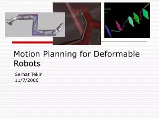
16. MOTION PLANNING FOR DEFORMABLE OBJECTS From slides by Ilknur Kaynar-Kabul

17. Introduction Algorithms so far the world was assumed to be made of rigid objects Why deformable objects? Deformable moving objects (wires, metal sheets) Deformable obstacles (e.g., human-body tissue structures) Need for physical model

18. First Paper:Planning paths for elastic objects under manipulation constraints (Lamiraux and Kavraki) Energy model

19. Second Paper:Probabilistic Roadmap Motion Planning for Deformable Objects(O. Burchan Bayazit, Jyh-Ming Lien, Nancy M.Amato)

20. Planning Paths for Elastic Objects Under Manipulation Constraints Florent Lamiraux Lydia E. Kavraki Rice University Int. J. Robotics Research, 2001.

21. Introduction • Goal: Plan paths for elastically deformable objects in a static environment • What is hard? • Representing the shape of an object with a possibly infinitely dimensional configuration space • Computing object shapes under actuator loading conditions • Collision checking for a shape-changing object

22. Problem Definition • What objects are considered? • Elastically deformable objects constrained by two actuators • Shape is determined by the lowest energy state for a given configuration of the actuators • Only the actuators are responsible for deformations (object cannot touch obstacles) ACTUATORS constrain the position of a subset of the points of the object

23. Problem Definition • In general, the configuration of an elastic object can be infinite-dimensional and cannot be represented by a vector • Configuration • Rest configuration q0 • Configuration q corresponds to mapping object through deformation Vq Vo Configuration q0 Configuration q

24. Problem Definition • Manipulation Constraints • Actuators constrain a subset of points V0p in V0 • Denote M as set of possible actuator positions and m is one of these positions in M • For all x in V0p there is a mapping Xm from V0 to Vq For a given position m of the actuators, points V0p are moved to Xm(V0p) The position of the other points of the objects should be such that the elastic energy of the object is minimized.

25. Problem Definition • Stable Equilibrium Configurations • Motion is slow enough to consider quasi-static paths – only stable equilibrium configurations • Stable equilibrium configurations are shapes at which the elastic energy is minimized Minimum Energy Cannot form this with two actuators

26. Problem Definition • Elastically Admissible Configurations • Elastic materials have a range of elastic deformation, large deformations may exceed this range and permanently deform • A range of elastic e(x) is defined for each point x • Admissible configurations are those in which e(x) is within the elastic range for all x in V0

27. Problem Definition • In path planning, “collision-free paths” are not enough – other conditions must be met • Manipulability: every point along the path must meet the actuator constraints • Quasi-static equilibrium: every point along the path must be in stable equilibrium (a minimum energy shape) • Elastic admissibility: no points along the path exceed the elastic limits of the material

28. Path Planning Algorithm • Algorithm • PRM approach is used, similar to conventional planners • Initial/Final configurations are chosen • Random free stable equilibrium configurations are chosen as nodes in roadmap • Nodes are connected by a local planner to form edges • Decompose deformation and position of object to save computing time

29. Path Planning Algorithm • Algorithm • The following steps are repeated until qinit and qgoal are in the same connected component of the roadmap: • Node generation • Node connection • Enhancement

30. Path Planning Algorithm • Node Generation • A random manipulator position is chosen and minimum energy shape calculated and admissibility is checked

31. Path Planning Algorithm • Node Generation • Random rigid-body motions are evaluated for collision-free configurations Rigid body motion is applied

32. Path Planning Algorithm • Node Generation • Random rigid-body motions are evaluated for collision-free configurations collision

33. Path Planning Algorithm • Node Generation • N collision-free configurations are found for the same deformation

34. Path Planning Algorithm • Node Connection • Each newly generated node is tested for connection with its K closest neighbors Distance function is evaluated

35. Path Planning Algorithm • Node Connection • Distance function should account for rigid body transformation and deformation Distance total = distance transformation + distance deformation

36. Path Planning Algorithm • Node Connection • Connections are performed by a deterministic local planner that generates quasi-static paths between pairs of configurations. Edges

37. Path Planning Algorithm • Node Connection • Local planner checks for collisions and admissibility Not a valid edge Violates elasticity limits Not a valid edge There exist collision

38. Path Planning Algorithm • Enhancement • Under the assumption that unconnected nodes are in difficult parts of the configuration space, add more nodes in these difficult areas

39. Path Planning Algorithm • Enhancement • Randomly walk away from unconnected nodes in the same configuration for a certain distance, reflecting off obstacles • A total of M enhancement nodes are added

40. Path Planning Algorithm • Path finding for a given qinit and qgoal • A graph search can yield a sequence of edges leading from qinit and qgoal • Concatenation of local paths results in a global path • We look for a path that minimizes the number of distinct deformations of the nodes of V belonging to the path -> reduce unnecessary deformations

41. Path Planning Algorithm • Distance Metric • Distance d(p,q) = dd(p,q) + dr(p,q) • dd is deformation distance, defined as the maximum distance a point moves in the local frame during a deformation • dr is rigid body translation and rotation distance, defined as the Euclidean distance in R6

42. Path Planning Algorithm • Collision Checking • With the decoupled motions, a standard collision checking algorithm can be applied, the research in this paper used RAPID (OBB-trees) • By keeping deformation separate from position, deformations can be stored and reused speeding up collision checking

43. Experimental Results • Bending Plate • 7 Dimensional problem • 6 for placement • 1 for deformation

44. Experimental Results • Bending Plate • The actuators are along the 2 opposite long edges • They are always parallel • Actuators constrain the distance d <= L between the opposite edges • Thus, deformation is one dimensional

45. Experimental Results • Bending Plate N = 200 K = 40 M = 100 Avg run time – 22.7 min Avg # nodes – 12,500

46. Experimental Results • Bending Plate • 9 Dimensional problem • 6 for placement • 3 for deformation

47. Experimental Results • Bending Plate • Manipulation constraints specify both the position and tangent direction of 2 opposite edges of the plate • One end of the curve is fixed and the other can move freely (translation along x1 and x3, rotation about x2)

48. Experimental Results • Bending Plate N = 200 K = 40 M = 100 Avg run time – 4 hrs 12 min Avg # nodes – 33,600

49. Experimental Results • Bending Plate Avg run time – 4 hrs 12 min • Space of deformation is of higher dimension • Large number of minimizations involved for computing deformation paths • The free space inside the box is constrained

50. Experimental Results • Elastic Pipe – one end fixed • 5 Dimensional problem • All 5 dimensions for deformation