Download
1 / 46
470 likes | 700 Vues
Inclusion and Exclusion Criteria (Defining the Study Population). General considerations Run-in periods (enrichment) Regression toward the mean. 2 e. . Regression Toward the Mean (Definition).

E N D
Inclusion and Exclusion Criteria(Defining the Study Population) • General considerations • Run-in periods (enrichment) • Regression toward the mean
2 e Regression Toward the Mean(Definition) • A variable extreme on its first measurement will be closer to the center of the distribution for a later measurement (on the average). • Results from within person variability (temporal variability and measurement error), i.e., .
Regression Towards the Mean Francis Galton, 1885, “Regression Towards Mediocrity in Hereditary Stature” Obs. Reg. Line Height of adult children Height of mid-parent “When mid-parents are taller than mediocrity, their children tend to be shorter than they.” “When mid-parents are shorter than mediocrity, their children tend to be taller than they.”
y = children’s height x = mid-parent’s height Regression Towards the Mean Regression towards the mean implies p<1
Suppose y = follow-up measurement of a response variable and x = baseline measurement of a response variable For example, if measurements are BP or serum cholesterol, p ≈ 0.70.
ExamplesStudies Comparing Ambulatoryand Office BP Measurements Normal volunteers 77 78 -1 (<90 mmHg) “Borderline Hypertensives” 96 93 3 (90 - 104 mmHg) “Established Hypertensives” 111 101 10 (≥105 mmHg) Pickering et al. “How common is white coat hypertension.” JAMA, 1988. Office DBP Awake DBP Difference
24-Hour Urine Sodium Excretionby Tertile of Excretion at BaselineControl Group in Mt. Sinai Hypertension Trial I 24 110.3 158.4 II 25 170.7 175.3 III 24 246.4 180.1 Baseline Mean 6-Month Mean Tertile N
Impact of Regression to the Meanin 3 Large Prevention Trials Screening Visit CPPT Cholesterol 292 281 – HDFP Diastolic BP 105 101 97 MRFIT Cholesterol 254 247 – DBP 99 91 91 Cigarettes/day 22 – 19 S1 S2 S3
MRFIT Screening andFollow-up Blood Pressures SI 99.2 80.5 -18.7 UC 99.2 83.6 -15.6 Screen 1 72 Months ∆
MRFIT Screening andFollow-up Blood Pressures SI 91.0 80.5 -10.5 UC 90.9 83.6 -7.3 Screen 2 and 3 72 Months ∆
Consider the following: - average level observed at screen 1 for those eligible at screen 1 - average level observed at screen 2 for those eligible at screen 1 - average of “true” level for those eligible at screen 1 - cut-point for eligibility at screen 1 - correlation between 2 observed values of risk measurement for individual Gardner and Heady, J Chron Dis, 1972
Assumptions = Observed risk factor level X = “True” risk level e = Error resulting from measurement of the risk factor and temporal variation = X + e E() = E(X) = X
Each person’s distribution Population distribution Individual A; long-term average below XC Individual B; long-term average above XC X XC Yudkin P, Lancet 1996
Solutions effect of regression toward the mean standardized cut-point for eligibility ordinate of standardized normal variable at zc . Prob (z ≤ z ) = area under standardized normal curve to the left of zc c
Z c f(z) -∞ 0 ∞ F(Z ) = Prob (Z ≤ Z ) c c
Solutions effect of regression toward the mean standardized cut-point for eligibility ordinate of standardized normal variable at zc . Prob (z ≤ z ) = area under standardized normal curve to the left of zc c
The following can be noted: s 2 1) If p = 1 or = 0, then no regression effect c c e 1 2 2) The smaller p , the greater the regression effect c c 1 2 2 s (the bigger the greater the regression effect). e c ¥ 3) With no selection, then f(z ) =0 ( = - ) and c c there is no regression effect.
Expected Regression to the Mean in Standard Deviation Units for Various Proportions Excluded in Screening and Levels of Correlation Proportion Excluded in Screening Correlation.01.05.25.50.60.70.80.85.90.95.99 0 .027 .108 .424 .798 .966 1.159 1.400 1.554 1.755 2.063 2.666 .10 .024 .098 .381 .718 .869 1.043 1.260 1.399 1.580 1.857 2.399 .20 .022 .087 .339 .638 .772 .927 1.120 1.244 1.404 1.650 2.132 .30 .019 .076 .297 .559 .676 .811 .980 1.088 1.229 1.444 1.866 .40 .016 .065 .254 .479 .579 .695 .840 .933 1.053 1.238 1.599 .50 .013 .054 .212 .399 .483 .579 .700 .777 .878 1.032 1.333 .60 .011 .043 .170 .319 .386 .463 .560 .622 .702 .825 1.066 .70 .008 .033 .127 .239 .290 .348 .420 .466 .527 .619 .800 .80 .005 .022 .085 .160 .193 .232 .280 .311 .351 .413 .533 .90 .003 .011 .042 .080 .097 .116 .140 .155 .176 .206 .267 Cutter G, Amer Stat 1976
Question 2: What are the expected levels at screen 1 and screen 2 for the lower and upper 1/3? What is an estimate of the regression effect?
Example #2CPPT Trial Use Gardner & Heady’s parameter estimates
Strategies for ReducingRegression Toward the Mean • Multiple measurements; multiple visits • Baseline free of selection • Standardization of methods; training
= total variability (n measurements per person) = inter-subject variability, and = intra-subject 2 2 x 2 e Choice of BaselineParticularly important in uncontrolled study NOTE: As n increases, expectations (1) and (2) get closer to one another. Therefore, averaging several readings and using the average to select subjects 1) reduces regression effect, and 2) results in selection of subjects with the risk factors closer to ”true” levels
2 2 x 2 e Consider CPPT Trial Example Again = 215 = 2225; =1600; = 625 p = 0.72 Suppose 3 screens are conducted for eligibility and average of 3 screening cholesterols is used for eligibility. x
Question: What is the average cholesterol at the 3 screens for those selected?
Question: What is the expected average at a subsequent visit for those eligible?
= 278 mg/dl vs. 268 mg/dl with 1 reading regression effect = 286-278 = 8 mg/dl compared with 21 mg/dl with 1 reading used for eligibility
1 2 3 Let = screen 1 level = screen 2 level = follow-up level Reference: Ederer, J Chronic Disease, 1972.
Impact of Regression to the Meanin 3 Large Prevention Trials Screening Visit CPPT Cholesterol 292 281 – HDFP Diastolic BP 105 101 97 MRFIT Cholesterol 254 247 – DBP 99 91 91 Cigarettes/day 22 – 19 S1 S2 S3
Other Consequences of Measurement Error/Short-Term Temporal Variability • Misclassification in application of eligibility criteria • Regression - dilution bias (see Clark R, Amer J Epid, 1999)
Treatment of Hypertensionin MRFIT and HDFP MRFIT 82 62 HDFP 100 75 Percent Treated in Experimental Group Projected Actual
Coronary Primary Prevention Trial Design(CPPT) Estimates of control group event rate (Pc) and experimental group event rate (Pe) determined based on Framingham Logistic Function STEPS: 1. Estimate logistic regression coefficient corresponding to total plasma cholesterol for endpoint CHD death or non-fatal MI in 7 years using Framingham men. 2. Calculate Pc for those men with total plasma cholesterol > 295 mg/dl (assume cholesterol is reduced 4% as a result of dietary advice). 3. Calculate Pe for same group of men assuming cholesterol is reduced by 28%.
CPPT Design Lipid Research Clinics Program: The Lipid Research Clinics Coronary Primary Prevention Trial: Design and Implementation. J Chronic Dis 32:609, 1979. For M risk eligible subjects with cholesterol (xi) > 295 mg/dL
No. of Visits (N) No. of Readings (M) ^ Coefficient (N,M) Expected (N,M) 1,1 (N,M / 1,1) ^ ^ ^ ^ Difference 1 1 0.0316 – – 2 0.0325 0.0330 -0.0005 2 1 0.0390 0.0385 0.0005 2 0.0419 0.0401 0.0018 Observed and Expected Logistic Regression Coefficients for Diastolic BP (mmHg) Endpoint: CHD Death (ICD-9 410-414) in 6 Years MRFIT Usual Care Men Not on Antihypertensive Treatment at Entry: 5211 Men; 70 CHD Deaths
Interpretation of Regression Coefficients for Measured Variables e.g., Diastolic BP Reduction in Risk Associated with 10 mm Hg Lower BP 1 Visit: 1 Reading: 1-e.0316(-10) = 1 - .729 = .271 27.1% reduction 2 Visits: 4 Readings: 1-e.0419(-10) = .342 34.2%
Mean Diastolic Blood Pressure (DBP) at “Baseline” (Survey 3, 1953-56) and at Subsequent Surveys 2 years and 4 years later for 5 categories of baseline DBP in 3,776 men and women in the Framingham Study. Mean DBP in each category (and difference between adjacent categories) Baseline DBP categories: mmHg Number of participants with repeat measurements 1: ≤79 1719 70.8 75.7 76.2 (12.9) (7.3) (7.7) 2: 80-89 1213 83.6 83.0 83.9 (9.9) (8.2) (7.4) 3: 90-99 566 93.5 91.2 91.3 (9.9) (8.0) (7.2) 4: 100-109 186 103.4 99.2 98.5 (13.0) (8.1) (6.2) 5: ≥110 92 116.4 107.3 104.7 Range of mean DBP 45.7 31.6 28.5 (ii) 2 years post-baseline (iii) 4 years post-baseline (i) at baseline MacMahon S, Lancet 1990
Conclusions 1. Regression towards the mean complicates the interpretation of many uncontrolled studies; frequently it is not recognized 2. In randomized clinical trials regression towards the mean can influence: • Cost, amount and nature of screening • Choice of baseline for within group comparisons • Hypothesized treatment effect (regression dilution bias)