Chapter 6 Relations
370 likes | 387 Vues
Explore various types of relations and their properties, like reflexive, symmetric, transitive. Learn how relationships are dealt with in everyday scenarios and problem-solving contexts.

Chapter 6 Relations
E N D
Presentation Transcript
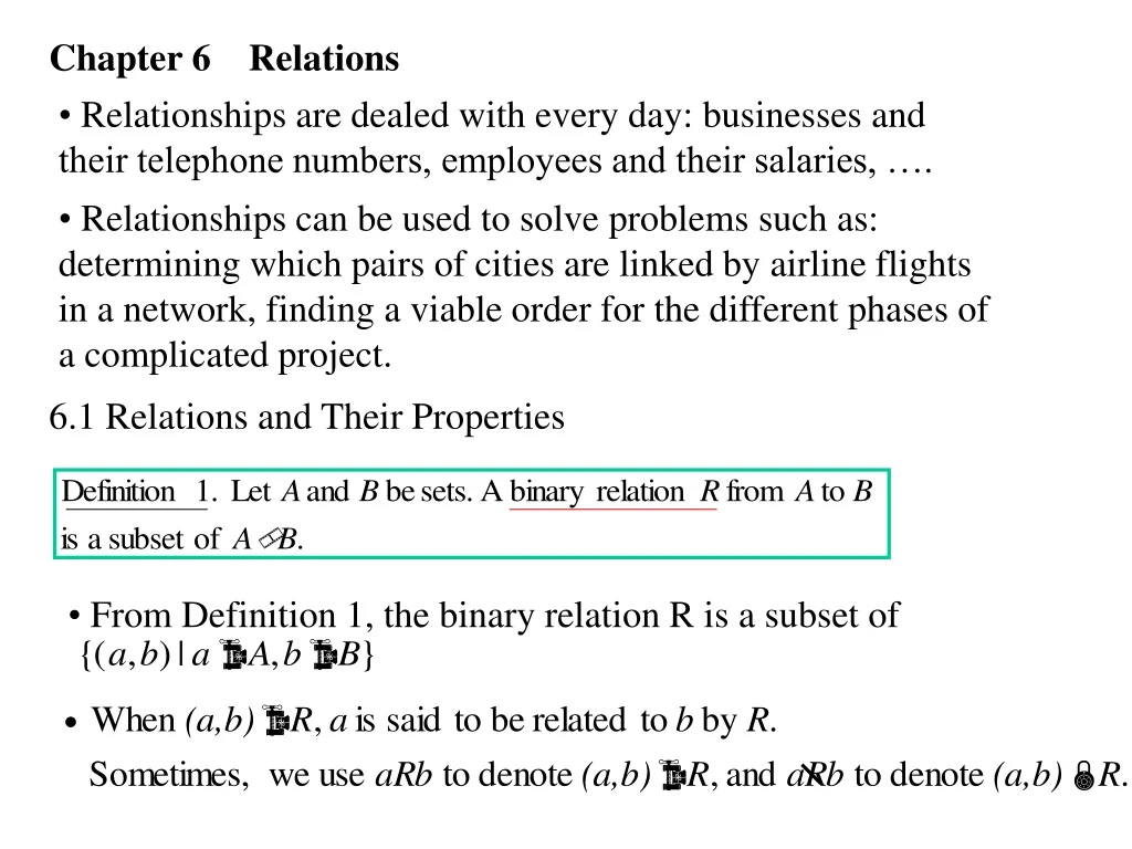
Chapter 6 Relations • Relationships are dealed with every day: businesses and their telephone numbers, employees and their salaries, …. • Relationships can be used to solve problems such as: determining which pairs of cities are linked by airline flights in a network, finding a viable order for the different phases of a complicated project. 6.1 Relations and Their Properties • From Definition 1, the binary relation R is a subset of
Example 1 Let A be the set of students, and let B the set of courses. Define R to be the relation that consists of those pairs (a,b), where a is a student enrolled in course b. Example 2 Let A be a set of all cities, and let B be the set of the 50 states in the United States. Define the relation R by specifying that (a,b) belongs to R if city a is in state b. Example 3 Let A={0,1,2} and B={a,b}.R={(0,a),(0,b),(1,a),(2,b)} is a relation from A to B. 0 a 1 b 2 Solution: R={(Boulder,Colorado),(Bangor,Maine),(Ann Arbor,Michigan), (Cupertino,California), (Red Bank,New Jersey),…}
0 a 1 b 2 0 a R R’ 1 b 2 Functions as Relations • A function f from a set A to a set B assigns a unique element of B to each element of A. But a relation does not have to be a function. Example Let A={0,1,2} and B={a,b}. Let R={(0,a),(0,b),(1,a),(2,b)} and R’={(0,a),(1,a),(2,b)} be two relations from A to B. R’ is a function, but R is not a function.
Definition 2. A relation R on the set A is a relation from A to A. Example 4. Let A be the set {1,2,3,4}. Which ordered pairs are in the relation R={(a,b) | a divides b}? Example 5. Consider the following relations on the set of integers. Relations on A Set Solution R={(1,1),(1,2),(1,3),(1,4),(2,2),(2,4),(3,3),(4,4)}.
Example 6. Consider the following relations on {1,2,3,4} Properties of Relations
Example 7. Consider the following relations on the set of integers. Example 8. Is the “divides” relation on the set of a positive integers reflexive? Solution: It is reflexive, since a|a whenever a is a positive integer.
Example 10. Consider the following relations on the set of integers. Example 11. Is the “divides” relation on the set of a positive integers symmetric? Is it antisymmetric? Solution: It is not symmetric, since 1|2, but 2|1. It is antisymmetric, since for any positive integers a and b with a|b and b|a, then a=b.
Example 13. Consider the following relations on the set of integers. Example 14. Is the “divides” relation on the set of a positive integers transitive? Solution: It is transitive, since a|b and b|c, then a|c, for any positive integers a,b,c.
Solution: R is reflexive, symmetric, and transitive, it is an equivalence relation. Example 2 Let R be the relation on the set of real numbers such that aRb if and only if a=b or a=-b. In Section 6.1, we showed that R is reflexive, symmetric, and transitive. It follows that R is an equivalence relation. 6.5 Equivalence Relations Definition 1. A relation on a set A is called an equivalence relation if it is reflexive, symmetric and transitive. • Two elements are related by an equivalence relation are called equivalent.
Example 3. Let R be the relation on the set of real numbers such that aRb if and only if a-b is an integer. Is R an equivalence relation? Solution: R is reflexive, symmetric and transitive. It is an equivalence relation.
Example 1 Show that the “greater than or equal” relation is a partial ordering one the set of integers. Example 2 Show that the divisibility relation (|) is a partial ordering on the set of positive integers. Example 3 Show that the inclusion relation ( ) is a partial ordering on the power set of a set S. 6.6 Partial Orderings Definition 1 A relation R on a set S is called a partial ordering or partial order if it is reflexive, antisymmetric, and transitive. A set S together with a partial ordering R is called a partially ordered set, and denoted by (S,R). A partial order R is also denoted as .
Example 4 Definition 3 If (S, ) is a partial ordering set and every two elements of S are comparable, S is called a totally ordered or linearly ordered set, and is called a total order or a linear order. Example 5 Example 6 Definition 2 The elements a and b of a partial ordering set (S, ) is called comparable if either a b or b a. When a and b are elements of S such that neither a b nor b a, a and b are called incomparable.
Definition 1 Let be the sets. An n-ary relation on these sets is a subset of are called as the domains of the relation and n is called as its degree. Primary key (no same value in the domain) Example 1 A student record are represented by 4-tuples of the form (student name, ID, Major, GPA). A sample database of six such record is: (Ackermann, 231455, Computer Sci, 3.88) (Adams, 888323, physics, 3.45) (Chou, 102147, Computer Sci, 3.49) (Goodfriend, 453876, Mathematics, 3.45) (Rao, 678543, Mathematics, 3.90) (Stevens, 786576, Psychology, 2.99) 6.7 n-ary Relations and Database A database consists of records, which are n-tuples, made up of fields. Table 1 Students
(C: GPA>3.5) Operations on n-ary relations Definition 2 Let R be an n-ary relation and C a condition that elements in R may satisfy. Then the selection operator maps the n-ary relation R to the n-ary relation of all n-tuples from R that satisfy the condition C.
Definition 3 The projection maps the n-tuple to the m-tuple , where
Definition 4 Let R be a relation of degree m and S a relation of degree n. The join where is a relation of degree m+n-p that consist of all (m+n-p)-tuples , where belongs to R and belongs to S. Student_name ID GPA ID Major GPA Ackermann Adams Chou Goodfriend Rao Stevens 231455 888323 102147 453876 678543 786576 3.88 3.45 3.49 3.45 3.90 2.99 231455 888323 102147 453876 678543 786576 Computer Sci Physics Computer Sci Mathematics Mathematics Psychology 3.88 3.45 3.49 3.45 3.90 2.99 R S
Chapter 7 Graphs San Francisco San Francisco Chicago Chicago New York New York Denver Denver Los Angeles Los Angeles Washington Washington Detroit Detroit San Francisco Chicago New York (2) multigraph Denver Washington Los Angeles Detroit (3) pseudograph Definition 1. (1) A simple undirectedgraph G=(V,E) consists of V, a nonempty set of vertices, and E, a set of unordered pairs of distinct elements of V called edges. (2) If more than one edges are allowed between two vertices, G is called multigraph. (3) If there is any edge connection the same vertex, G is called pseudograph. (1) Simple undirected graph V={San Francisco, Los Angles, Denver, Chicago, Detroit, Washington, New York} E={(San Francisco, Los Angeles), (San Francisco,Denver), (Los Angeles,Denver), (Denver,Chicago), (Chicago,Detroit), (Chicago,New York), (Chicago,Washington), (Detroit,New York), (Washington,New York)}
New York Example 1 Precedence Graphs and Concurrent Processing F E A a:=0 B b:=1 C c:=a+1 D d:=b+a E e:=d+1 F e:=c+d C D Detroit A B San Francisco Chicago Denver Los Angeles Washington Definition 2. A directed graph G=(V,E) consists of V, a nonempty set of vertices, and E, a set of ordered pairs of distinct elements of V called edges.
Definition 3. • Let e=(u,v)be an edge of Graph G (undirected or directed). (i)Vertices u and v are called adjacent in G. • (ii)Edge e is called incident with (or connect) the vertices u and v. • The degree of a vertex v in an undirected graph is the number of edges incident with it, denoted by deg(v). • Let e=(u,v) be an edge of a directed graph G. The vertex u is called the initial vertex of (u,v), and v is called the terminal vertex of (u,v). • 4. Let v be a vertex of directed graph G. The in-degree of v is the number of edges with v as their terminal vertex. The out-degree of v is the number of edges with b as their initial vertex.
Connectivity Definition 4. Given a graph G=(V,E), a path of G is a sequence of vertices E F C D A B H I E F C D A B H I
E F C D Connected graph Unconnected graph A B H I E F E E F F Not Strongly connected C Strongly connected C C D D D A B A A H I Definition 5. An undirected graph is called connected if there is a path between every pair of distinct vertices of the graph. Definition 6. A directed graph is strongly connected if there is a path from a to b whenever a and b are the vertices in the graph.
Example 1 Which of the graphs are trees? Chapter 8 Trees 8.1 Introduction to tree Definition 1. A tree is a connected undirected graph with no simple circuits. Theorem 1 Au undirected graph is a tree if and only if there is a unique simple path between any two of its vertices.
root parent subtree third child Left child Right child Right subtree Left subtree Ordered rooted tree Binary tree (every node has at most two children)
8.3 Tree Traversal Ordered rooted trees are used to store information. We need procedures for visiting each vertex of and ordered rooted tree to access data. Root of T 15 6 18 19 30 9 20 19 1 7 17 21 4 13 5 4 19 11 The preorder traversal of T 15,6,9,30,21,4,7,13,11,18,17,1,19,20,19,19,4,5
Root of T 15 6 18 19 30 9 20 19 1 7 17 21 4 13 5 4 19 11 The inorder traversal of T 9,6,21,30,4,11,13,7,15,17,18,1, 20,19,19,19,4,5
Root of T 15 6 18 19 30 9 20 19 1 7 17 21 4 13 5 4 19 11 The postorder traversal of T 9,21,4,30,11,13,7,6,17,1,18,20,19,4,5,19,19,15
root 15 6 18 3 7 17 20 13 1 4 9 8.2 Application of Trees Binary Search Tree • Definition 1 Binary Search Tree is a Binary Tree satisfying the following condition: • Each vertex contains an item with an key which belongs to a total ordering set and two links to its left child and right child, respectively. • In each node, its key is larger than the keys of all vertices in its left subtree and smaller than the keys of all the vertices in its right subtree. Operations in a BST Search (given a key return the corresponding data if it is in the BST) Insert (given a data insert it into the BST) Delete (given a key delete the corresponding data from BST) key
A node of BST: item, right child, left child item (key/other data) Right left root 65/data A BST 30/data 75/data class Node{ item Item; Node Left; Node Right; } struct item { int id; string name; float grade; } 25/data / 45/data 68/data / / 80/data 20/data / / 40/data 55/data / 78/data / / 88/data / / 35/data / 60/data / / 42/data / / 38/data key 36/data / / 39/data / / Define a node of BST
root 65/data A BST 30/data 75/data 25/data / 45/data 68/data / / 80/data 20/data / / 40/data 55/data / 78/data / / 88/data / / 35/data / 60/data / / 42/data / / 38/data 36/data / / 39/data / / Visit the nodes of BST in-order Procedure InOrder(Node root) { if (root ≠ null)) { InOrder(root.Left); visit root; InOrder(root.Right); } } In-order visit in the BST (only show keys): 20,25,30,35,36,38,39,40,42,45,55,60,65,68,75,78,80,88 A BST can be visited in three ways: in-order, pre-order and post-order
height root 65/data A BST 30/data 75/data 25/data / 45/data 68/data / / 80/data 20/data / / 40/data 55/data / 78/data / / 88/data / / 35/data / 60/data / / 42/data / / 38/data 36/data / / 39/data / / Operation 1: Search Operation 1: Search Procedure Search(int id) { Node x = root; while (x ≠ null and x.Item.id ≠ key ) { if (id < x.Item.id) x = x.Left; else x = x.Right; } return x; /* x.id = key or x = null */ } • Time Complexity • O(height of BST) • Average case: O(lg n) • Worst case O(n) • where n is the size of the BST Example: Search (42) Search (64)
root A BST height 65/data 30/data 75/data 25/data / 45/data 68/data / / 80/data 20/data / / 40/data 55/data / 78/data / / 88/data / / 35/data / 60/data / / 42/data / / 62/data / / 38/data 36/data / / 39/data / / Operation 2: Insert Procedure Insert( item newItem) { Node newNode: = new Node(newItem); Node parent = null; Node current = root; while (current ≠ null) { parent: = current; if (newNode.Item.id < current.Item.id) current: = current.Left; else current: = current.Right; } if (parent = null) root: = newNode; else { if (newNode.Item.id < parent.Item.id) parent.Left: = newNode; else parent.Right: = newNode; } } current parent curr paren curr paren curr paren curr paren curr = null • Time Complexity • O(height of BST) • Average case: O(lg n) • Worst case: O(n) • where n is the size of the BST Insert Create a new node for new item (e.g., 62/data) Find the place for insertion Link the new node
height root 65/data 30/data 75/data 25/data / 45/data 68/data / / 80/data 20/data / / 40/data 55/data / 78/data / / 88/data / / 35/data / 60/data / / 42/data / / 38/data 36/data / / 39/data / / Operation 3: Delete Case 1: Deleting node (current) has no child A BST Example: Delete the node with item (36/data) if (current.Left = null and current.Right: = null) { if (current = root)root: = null; else if (parent.left = current) parent.Left: = null; elseparent.Right = null; } • Time Complexity • Find the deleting node (current) and its parent: O(height of BST) • Delete current: O(1) • Therefore, the time complexity for case 1 is O(height of BST) • Average case: O(lg n) • Worst case: O(n) • where n is the size of the BST parent current Delete Find the deleting node (current) and its parent Delete current The first step is similar to Search. We only consider the step of delete current.
height root 65/data 30/data 75/data 25/data / 45/data 68/data / / 80/data 20/data / / 40/data 55/data / 78/data / / 88/data / / 35/data / 60/data / / 42/data / / 38/data 36/data / / 39/data / / Case 2: Deleting node (current) has one child Operation 3: Delete Example: delete the node with item (35/data) ABST if (current.Left = null or current.Right = null) { if (current.Right = null) if (current = root)root: = current.Left; else if (parent.Left = current) parent.Left: = current.Left; else parent.Right: = current.Left; else if (current.Left = null) if (current = root)root: = current.Right; else if (parent.Left = current) parent.Left: = current.Right; else parent.Right: = current.Right; } parent current • Time Complexity • Find the deleting node (current) and its parent: O(height of BST) • Delete current: O(1) • Therefore, the time complexity for case 1 is O(height of BST) • Average case: O(lg n) • Worst case: O(n) • where n is the size of the BST Delete Find the deleting node (current) and its parent Delete current The first step is similar to Search. We only consider the step of delete current.
height Operation 3: Delete Case 3: Deleting node (current) has two children root ABST 65/data Example: delete the node with item (30/data) current 75/data Step 1 and 2 are similar to Search. We only consider step 3 and 4. 30/data 25/data / 45/data 68/data / / 80/data if (!(successor == current.Right)) sucessorParent.Right = successor.Right; current.item = successor.item Succ Parent 20/data / / 40/data 55/data / 78/data / / 88/data / / successor • Time Complexity • Find the deleting node (current) and its parent: O(height of BST) • Find successor and successor’s parent: O(height of BST) • Link successor’s parent to successor.Right: O(1) • Replace the current.item by successor.item: O(1) • Therefore, the time complexity for case 1 is O(height of BST) • Average case: O(lg n) • Worst case: O(n) • where n is the size of the BST 35/data / 35/data 60/data / / 42/data / / 38/data 36/data / / 39/data / / Delete Find the deleting node (current) and its parent Find successor which is the node with the smallest key in current’s left, and successor’s parent. Link successorParent to successor.Right Replace the current.item by successor.item
Example 1 Form a binary search tree for the words mathematics, physics, geography, zoology, meteorology, geology, psychology, and chemistry (using alphabetical order). Example 2 Find the item with key Zoology in the tree of Example 1. Example 3 Insert the item with key English in the tree of Example 2. Example 4 Delete the item with key English in the tree of Example 3.