Download

1 / 21
210 likes | 242 Vues
Learn about the robust and real-time face detection technique developed by Viola and Jones in 2002, focusing on feature selection with AdaBoost and Cascade algorithms. Understand the integral image representation and the efficient detection of faces in images.

E N D
Robust Real-time Face DetectionbyPaul Viola and Michael Jones, 2002 Presentation by Kostantina Palla & Alfredo Kalaitzis School of Informatics University of Edinburgh February 20, 2009
Overview • Robust – very high Detection Rate (True-Positive Rate) & very low False-Positive Rate… always. • Real Time – For practical applications at least 2 frames per second must be processed. • Face Detection – not recognition. The goal is to distinguish faces from non-faces (face detection is the first step in the identification process)
Face Detection • Can a simple feature (i.e. a value) indicate the existence of a face? • All faces share some similar properties • The eyes region is darker than the upper-cheeks. • The nose bridge region is brighter than the eyes. • That is useful domain knowledge • Need for encoding of Domain Knowledge: • Location - Size: eyes & nose bridge region • Value: darker / brighter
Overview | Integral Image | AdaBoost| Cascade Rectangle features • Rectangle features: • Value = ∑ (pixels in black area) - ∑ (pixels in white area) • Three types: two-, three-, four-rectangles, Viola&Jones used two-rectangle features • For example: the difference in brightness between the white &black rectangles over a specific area • Each feature is related to a special location in the sub-window • Each feature may have any size • Why not pixels instead of features? • Features encode domain knowledge • Feature based systems operate faster
Relevant feature Irrelevant feature Overview | Integral Image| AdaBoost| Cascade Feature selection • Problem: Too many features • In a sub-window (24x24) there are ~160,000 features (all possible combinations of orientation, location and scale of these feature types) • impractical to compute all of them (computationally expensive) • We have to select a subset of relevant features – which are informative - to model a face • Hypothesis: “A very small subset of features can be combined to form an effective classifier” • How? • AdaBoost algorithm
Overview | Integral Image| AdaBoost| Cascade AdaBoost • Stands for “Adaptive” boost • Constructs a “strong” classifier as a linear combination of weighted simple “weak” classifiers Weak classifier Strong classifier Image Weight
AdaBoost – Feature Selection Problem On each round, large set of possible weak classifiers (each simple classifier consists of a single feature) – Which one to choose? choose the most efficient (the one that best separates the examples – the lowest error) choice of a classifier corresponds to choice of a feature At the end, the ‘strong’ classifier consists of T features Adaboost’s solution AdaBoost searches for a small number of good classifiers – features (feature selection) adaptively constructs a final strong classifier taking into account the failures of each one of the chosen weak classifiers (weight appliance) AdaBoost is used to both select a small set of features and train a strong classifier Overview | Integral Image| AdaBoost| Cascade
Overview | Integral Image| AdaBoost| Cascade AdaBoost - Getting the idea… • Given: example images labeled +/- • Initially, all weights set equally • Repeat T times • Step 1: choose the most efficient weak classifier that will be a component of the final strong classifier (Problem! Remember the huge number of features…) • Step 2: Update the weights to emphasize the examples which were incorrectly classified • This makes the next weak classifier to focus on “harder” examples • Final (strong) classifier is a weighted combination of the T “weak” classifiers • Weighted according to their accuracy
Overview | Integral Image| AdaBoost| Cascade AdaBoost example • AdaBoost starts with a uniform distribution of “weights” over training examples. • Select the classifier with the lowest weighted error (i.e. a “weak” classifier) • Increase the weights on the training examples that were misclassified. • (Repeat) • At the end, carefully make a linear combination of the weak classifiers obtained at all iterations. Slide taken from a presentation by Qing Chen, Discover Lab, University of Ottawa
Overview | Integral Image| AdaBoost| Cascade Now we have a good face detector • We can build a 200-feature classifier! • Experiments showed that a 200-feature classifier achieves: • 95% detection rate • 0.14x10⁻³ FP rate (1 in 14084) • Scans all sub-windows of a 384x288 pixel image in 0.7 seconds (on Intel PIII 700MHz) • The more the better (?) • Gain in classifier performance • Lose in CPU time • Verdict: good & fast, but not enough • 0.7 sec / frame IS NOT real-time.
Integral Image Representation(also check back-up slide #1) Given a detection resolution of 24x24 (smallest sub-window), the set of different rectangle features is ~160,000 ! Need for speed Introducing Integral Image Representation Definition: The integral image at location (x,y), is the sum of the pixels above and to the left of (x,y), inclusive The Integral image can be computed in a single pass and only once for each sub-window! Overview | Integral Image | AdaBoost| Cascade x y
Overview | Integral Image | AdaBoost| Cascade IMAGE INTEGRAL IMAGE
Rapid computation of rectangular features Using the integral image representation we can compute the value of any rectangular sum (part of features) in constant time For example the integral sum inside rectangle D can be computed as:ii(d) + ii(a) – ii(b) – ii(c) two-, three-, and four-rectangular features can be computed with 6, 8 and 9 array references respectively. As a result: feature computation takes less time Overview | Integral Image | AdaBoost| Cascade ii(a) = A ii(b) = A+B ii(c) = A+C ii(d) = A+B+C+D D = ii(d)+ii(a)-ii(b)-ii(c)
Overview | Integral Image| AdaBoost| Cascade The attentional cascade • On average only 0.01% of all sub-windows are positive (are faces) • Status Quo: equal computation time is spent on all sub-windows • Must spend most time only on potentially positive sub-windows. • A simple 2-feature classifier can achieve almost 100% detection rate with 50% FP rate. • That classifier can act as a 1st layer of a series to filter out most negative windows • 2nd layer with 10 features can tackle “harder” negative-windows which survived the 1st layer, and so on… • A cascade of gradually more complex classifiers achieves even better detection rates. On average, much fewer features are computed per sub-window (i.e. speed x 10)
Step 1 … Step 4 … Step N
Face Detection: Visualized • http://vimeo.com/12774628
Training a cascade of classifiers Overview | Integral Image| AdaBoost| Cascade • Given the goals, to design a cascade we must choose: • Number of layers in cascade (strong classifiers) • Number of features of each strong classifier (the ‘T’ in definition) • Threshold of each strong classifier (the in definition) • Optimization problem: • Can we find optimum combination?
A simple framework for cascade training Overview | Integral Image| AdaBoost| Cascade • Do not despair. Viola & Jones suggested a heuristic algorithm for the cascade training: • does not guarantee optimality • but produces a “effective” cascade that meets previous goals • Manual Tweaking: • overall training outcome is highly depended on user’s choices • select fi (Maximum Acceptable False Positive rate / layer) • select di (Minimum Acceptable True Positive rate / layer) • select Ftarget (Target Overall FP rate) • possible repeat trial & error process for a given training set • Until Ftarget is met: • Add new layer: • Until fi , di rates are met for this layer • Increase feature number & train new strong classifier with AdaBoost • Determine rates of layer on validation set
Cascade Training Overview | Integral Image| AdaBoost| Cascade
Training phase Cascade trainer Classifier cascade framework Integral Representation Training Set (sub-windows) Strong Classifier 1 (cascade stage 1) Feature computation Strong Classifier 2 (cascade stage 2) AdaBoost Feature Selection Strong Classifier N (cascade stage N) Overview | Integral Image| AdaBoost| Cascade Testing phase FACE IDENTIFIED
pros … • Extremely fast feature computation • Efficient feature selection • Scale and location invariant detector • Instead of scaling the image itself (e.g. pyramid-filters), we scale the features. • Such a generic detection scheme can be trained for detection of other types of objects (e.g. cars, hands) … and cons • Detector is most effective only on frontal images of faces • can hardly cope with 45o face rotation • Sensitive to lighting conditions • We might get multiple detections of the same face, due to overlapping sub-windows.