Face Detection using the Viola-Jones Method
CS 175, Fall 2007 Padhraic Smyth Department of Computer Science University of California, Irvine. Face Detection using the Viola-Jones Method . Outline. Viola Jones face detection algorithm State-of-the-art face detector MATLAB code available for CS 175 for implementing this algorithm

Face Detection using the Viola-Jones Method
E N D
Presentation Transcript
CS 175, Fall 2007 Padhraic Smyth Department of Computer Science University of California, Irvine Face Detection using the Viola-Jones Method
Outline • Viola Jones face detection algorithm • State-of-the-art face detector • MATLAB code available for CS 175 for implementing this algorithm • See viola_jones.zip, under projectcode on the class Web page
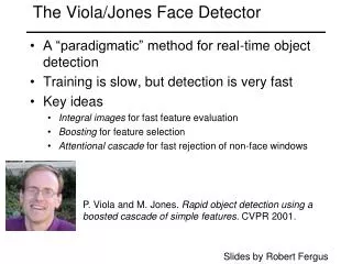
Viola-Jones Face Detection Algorithm Overview : Viola Jones technique overview Features Integral Images Feature Extraction Weak Classifiers Boosting and classifier evaluation Cascade of boosted classifiers Example Results Full details available in paper by Viola and Jones, International Journal of Computer Vision, 2004 Some of the following slides were adapted from a presentation by Nathan Faggian
Viola Jones Technique Overview Three major contributions/phases of the algorithm : Feature extraction Classification using boosting Multi-scale detection algorithm Feature extraction and feature evaluation. Rectangular features are used, with a new image representation their calculation is very fast. Classifier training and feature selection using a slight variation of a method called AdaBoost. A combination of simple classifiers is very effective
Features Four basic types. They are easy to calculate. The white areas are subtracted from the black ones. A special representation of the sample called the integral image makes feature extraction faster.
Integral images Summed area tables A representation that means any rectangle’s values can be calculated in four accesses of the integral image.
Feature Extraction Features are extracted from sub windows of a sample image. The base size for a sub window is 24 by 24 pixels. Each of the four feature types are scaled and shifted across all possible combinations In a 24 pixel by 24 pixel sub window there are ~160,000 possible features to be calculated.
Learning with many features • We have 160,000 features – how can we learn a classifier with only a few hundred training examples without overfitting? • Idea: • Learn a single simple classifier • Classify the data • Look at where it makes errors • Reweight the data so that the inputs where we made errors get higher weight in the learning process • Now learn a 2nd simple classifier on the weighted data • Combine the 1st and 2nd classifier and weight the data according to where they make errors • Learn a 3rd classifier on the weighted data • … and so on until we learn T simple classifiers • Final classifier is the combination of all T classifiers • This procedure is called “Boosting” – works very well in practice.
Recall: Perceptron Operation • Equations of “thresholded” operation: = 1 (if w1x1 +… wd xd + wd+1 > 0) o(x1, x2,…, xd-1, xd) = -1 (otherwise)
Perceptron with just a Single Feature • Equations of “thresholded” operation: • Equivalent to x1 > - wd+1 / w1 i.e., equivalent to comparing the feature to a threshold Learning = finding the best threshold for a single feature Can be trained by gradient descent (or direct search) = 1 (if w1x1 + wd+1 > 0) o(x1) = -1 (otherwise)
Boosting with Single Feature Perceptrons • Viola-Jones version of Boosting: • “simple” (weak) classifier = single-feature perceptron • see last slide • With K features (e.g., K = 160,000) we have 160,000 different single-feature perceptrons • At each stage of boosting • given reweighted data from previous stage • Train all K (160,000) single-feature perceptrons • Select the single best classifier at this stage • Combine it with the other previously selected classifiers • Reweight the data • Learn all K classifiers again, select the best, combine, reweight • Repeat until you have T classifiers selected • Hugely computationally intensive • Learning K perceptrons T times • E.g., K = 160,000 and T = 1000
How is classifier combining done? • At each stage we select the best classifier on the current iteration and combine it with the set of classifiers learned so far • How are the classifiers combined? • Take the weight*feature for each classifier, sum these up, and compare to a threshold (very simple) • Boosting algorithm automatically provides the appropriate weight for each classifier and the threshold • This version of boosting is known as the AdaBoost algorithm • Some nice mathematical theory shows that it is in fact a very powerful machine learning technique
Cascade of Boosted Classifiers Referred here as a degenerate decision tree. Very fast evaluation. Quick rejection of sub windows when testing. Reduction of false positives. Each node is trained with the false positives of the prior. AdaBoost can be used in conjunction with a simple bootstrapping process to drive detection error down. Viola and Jones present a method to do this, that iteratively builds boosted nodes, to a desired false positive rate.
Detection in Real Images • Basic classifier operates on 24 x 24 subwindows • Scaling: • Scale the detector (rather than the images) • Features can easily be evaluated at any scale • Scale by factors of 1.25 • Location: • Move detector around the image (e.g., 1 pixel increments) • Final Detections • A real face may result in multiple nearby detections • Postprocess detected subwindows to combine overlapping detections into a single detection
Training In paper, 24x24 images of faces and non faces (positive and negative examples).
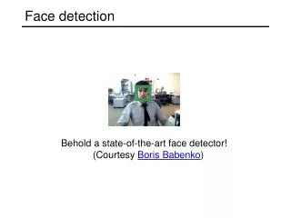
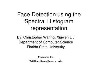
Sample results using the Viola-Jones Detector Notice detection at multiple scales
Practical implementation • Details discussed in Viola-Jones paper • Training time = weeks (with 5k faces and 9.5k non-faces) • Final detector has 38 layers in the cascade, 6060 features • 700 Mhz processor: • Can process a 384 x 288 image in 0.067 seconds (in 2003 when paper was written)
Code and Data for CS 175 • In directory viola_jones.zip (under MATLAB code for Projects) • Code has been written by Nathan (TA) • Current “release” is not complete – he will be updating it • Please email Nathan for questions/help/discussion in using this code (nsutter@ics.uci.edu) • Major components: • Feature extraction (written) • Boosting algorithm (written) • Cascade (not written – may not be necessary) • Multi-scale multi-location detection (not written)
Code and Data for CS 175 • Look at MATLAB directory on the Web page to see what functions and data are available
Summary • Viola-Jones face detection • Features • Integral Images • Feature Extraction • Weak Classifiers • Boosting and classifier evaluation • Cascade of boosted classifiers • Example Results • MATLAB code available on the class Web site • Will likely require some emails with Nathan to figure out how to use it • Work on your projects! Progress report due a week from Monday.