Download
1 / 30
320 likes | 683 Vues
Cos 429: Face Detection (Part 2) Viola-Jones and AdaBoost Guest Instructor: Andras Ferencz (Your Regular Instructor: Fei-Fei Li) Thanks to Fei-Fei Li, Antonio Torralba, Paul Viola, David Lowe, Gabor Melli (by way of the Internet) for slides. Face Detection. Face Detection. Sliding Windows.

E N D
Cos 429: Face Detection (Part 2) Viola-Jones and AdaBoostGuest Instructor: Andras Ferencz(Your Regular Instructor: Fei-Fei Li)Thanks to Fei-Fei Li, Antonio Torralba, Paul Viola, David Lowe, Gabor Melli (by way of the Internet) for slides
Sliding Windows 1. hypothesize: try all possible rectangle locations, sizes 2. test: classify if rectangle contains a face (and only the face) Note: 1000's more false windows then true ones.
Background Faces In some feature space Classification (Discriminative)
Image Features 4 Types of “Rectangle filters” (Similar to Haar wavelets Papageorgiou, et al. ) Based on 24x24 grid:160,000 features to choose from g(x) = sum(WhiteArea) - sum(BlackArea)
Image Features F(x) = α1 f1(x) + α2 f2(x) + ... 1 if gi(x) > θi -1 otherwise fi(x) = Need to: (1) Select Features i=1..n, (2) Learn thresholds θi , (3) Learn weights αi
Why rectangle features? (1)The Integral Image • The integral image computes a value at each pixel (x,y) that is the sum of the pixel values above and to the left of (x,y), inclusive. • This can quickly be computed in one pass through the image (x,y)
Why rectangle features? (2)Computing Sum within a Rectangle • Let A,B,C,D be the values of the integral image at the corners of a rectangle • Then the sum of original image values within the rectangle can be computed: sum = A – B – C + D • Only 3 additions are required for any size of rectangle! • This is now used in many areas of computer vision D B A C
Boosting How to select the best features? How to learn the classification function? F(x) = α1 f1(x) + α2 f2(x) + ....
Defines a classifier using an additive model: Boosting Strong classifier Weak classifier Weight Features vector
+1 ( ) yt = -1 ( ) Boosting • It is a sequential procedure: xt=1 Each data point has a class label: xt xt=2 and a weight: wt =1
+1 ( ) yt = -1 ( ) Toy example Weak learners from the family of lines Each data point has a class label: and a weight: wt =1 h => p(error) = 0.5 it is at chance
+1 ( ) yt = -1 ( ) Toy example Each data point has a class label: and a weight: wt =1 This one seems to be the best This is a ‘weak classifier’: It performs slightly better than chance.
+1 ( ) yt = -1 ( ) Toy example Each data point has a class label: We update the weights: wt wt exp{-yt Ht} We set a new problem for which the previous weak classifier performs at chance again
+1 ( ) yt = -1 ( ) Toy example Each data point has a class label: We update the weights: wt wt exp{-yt Ht} We set a new problem for which the previous weak classifier performs at chance again
+1 ( ) yt = -1 ( ) Toy example Each data point has a class label: We update the weights: wt wt exp{-yt Ht} We set a new problem for which the previous weak classifier performs at chance again
+1 ( ) yt = -1 ( ) Toy example Each data point has a class label: We update the weights: wt wt exp{-yt Ht} We set a new problem for which the previous weak classifier performs at chance again
Toy example f1 f2 f4 f3 The strong (non- linear) classifier is built as the combination of all the weak (linear) classifiers.
1. Train learner ht with min error 2. Compute the hypothesis weight 3. For each example i = 1 to m Output AdaBoost Algorithm Given: m examples (x1, y1), …, (xm, ym) wherexiÎX, yiÎY={-1, +1} The goodness of ht is calculated over Dt and the bad guesses. Initialize D1(i) = 1/m For t = 1 to T The weight Adapts. The bigger et becomes the smaller at becomes. Boost example if incorrectly predicted. Zt is a normalization factor. Linear combination of models.
Boosting with Rectangle Features • For each round of boosting: • Evaluate each rectangle filter on each example (compute g(x)) • Sort examples by filter values • Select best threshold (θ) for each filter (one with lowest error) • Select best filter/threshold combination from all candidate features (= Feature f(x)) • Compute weight (α) and incorporate feature into strong classifier F(x) F(x) + α f(x) • Reweight examples
by minimizing the exponential loss Boosting Boosting fits the additive model Training samples The exponential loss is a differentiable upper bound to the misclassification error.
Exponential loss Squared error Loss 4 Misclassification error 3.5 Squared error 3 Exponential loss 2.5 2 Exponential loss 1.5 1 0.5 0 -1.5 -1 -0.5 0 0.5 1 1.5 2 yF(x) = margin
Sequential procedure. At each step we add Boosting to minimize the residual loss input Desired output Parameters weak classifier For more details: Friedman, Hastie, Tibshirani. “Additive Logistic Regression: a Statistical View of Boosting” (1998)
Example Classifier for Face Detection A classifier with 200 rectangle features was learned using AdaBoost 95% correct detection on test set with 1 in 14084 false positives. Not quite competitive... ROC curve for 200 feature classifier
% False Pos 0 50 vs false neg determined by 50 100 % Detection T T T T IMAGE SUB-WINDOW Classifier 2 Classifier 3 FACE Classifier 1 F F F F NON-FACE NON-FACE NON-FACE NON-FACE Building Fast Classifiers • Given a nested set of classifier hypothesis classes • Computational Risk Minimization
Cascaded Classifier 50% 20% 2% • A 1 feature classifier achieves 100% detection rate and about 50% false positive rate. • A 5 feature classifier achieves 100% detection rate and 40% false positive rate (20% cumulative) • using data from previous stage. • A 20 feature classifier achieve 100% detection rate with 10% false positive rate (2% cumulative) IMAGE SUB-WINDOW 5 Features 20 Features FACE 1 Feature F F F NON-FACE NON-FACE NON-FACE
Solving other “Face” Tasks Profile Detection Facial Feature Localization Demographic Analysis