A fast Prunning Algorithm for optimal Sequence Alignment
A fast Prunning Algorithm for optimal Sequence Alignment. Linear Space Bounded Dynamic Programming. Overview. An introduction to alignments Dynamic Programming Other approaches to optimal alignment calculation A*-star algorithm LBD and boundaries Results Outlook on coming improvements.

A fast Prunning Algorithm for optimal Sequence Alignment
E N D
Presentation Transcript
A fast Prunning Algorithm for optimal Sequence Alignment Linear Space Bounded Dynamic Programming
Overview • An introduction to alignments • Dynamic Programming • Other approaches to optimal alignment calculation • A*-star algorithm • LBD and boundaries • Results • Outlook on coming improvements
Alignments • “the holy grail of Bioinformatics“ – Dan Gusfield • sequencing • function of genes and proteins • structure of proteins • evolutionary trees Sequencing gel
Mathematical Formalization • Given k sequences sk over an alphabet Σ and k sequences ask over an extended alphabet Σ΄ = Σ + {-} • The set A = {as1, as2, ..., ask} is a sequence alignment when each of the following three conditions are fullfilled • Each of the sequences in A have the same length • If you remove the gap symbols you arrive at the original sequneces • There is no column of gap symbols AGGTCG AGAC_ G ACGC_ G AGGTCG AGACG ACGCG
Dynamic Programming • Algorithm for finding the optimal sequence alignment: Needleman–Wunsch algorithm AGC_G A_CGG AGCG_ A_CGG
Dynamic Programming • Analysis of the Algorithm • Runtime: O(n*n) (filling a quadratic matrix) • Space consumption: O(n*n) (store n * n entries of the quadratic matrix) • Comparison of the genomes of Yeast, Saccharomyces cerevisiae (20 * 10^6bp) Fruit fly, Drosophila melanogaster (130 * 10^6bp) Space consumption: 20*10^6 * 130 * 10^6 = 26 * 10 ^14 4 Bytes to store an integer => 26 * 10 ^5 Gigabytes Drosophila melanogaster Saccharomyces cerevisiae
Hirschberg‘s Divide & Conquer • Main idea: • Only the row above neccessary to compute the one below that • Problem: Backtracking is not possible anymore • Algorithm: • Divide s1 in s1a and s1b • Align s1a with s2 and s1b with s2 • Search the largest transition (maximum sum) of these rows. • Go in recursion • Extra cell computations but space requirements reduced to O(n^d-1) s1a s1b s2 s1a s1b s2
A*-Algorithm • A classic graph algorithm to find the shortest distance between two locations
A*-Algorithm • Mathematical formalization • Scoring function f*(n) = g*(n) + h*(n) with g* giving the optimal path to node n found so far and the heuristic h* giving an optimistic approximation for the cost of a path from node n to a goal node • h* may never under-/overerstimate the score! • Open list/priority que, close list (avoid circles)
A*- Algorithm • Application • The shortest path problem • Use coordinate frame as the heuristic (shortest connection between to points is a straight line) • Alignments • Problems • Close and open list can easily become large • Not applicable to our problem in the basic version • Extensions • Do not store close list • Do not insert none promising children in open lists
Bounded Dynamic Programming • Main idea: Combine the low overhead of dynamic programming with the pruning capabilities of A* • Algorithm(1) • Only prune where promising • Compute the matrix (anti-)diagonalwise and check for pruning always at the end of the diagonal which means to compare the current upper bound with the lowest lower bound • Good upper and lower bounds are neccessary Diagonal wise computation & pruning pruned matrix
Upper and lower Bounds • Lower Bounds • Diagonal Alignment e.g align the sequences directly without any gaps • Greedy headlight search • Result of several local alignments • Always search the frontier for the largest value • Use this as a fulcrum for the next local alignment step • Only use diagonals for computing as no backtracking is needed • Size of local alignment influences the time consumption drastically Greedy headlight search
Upper and lower Bounds • Upper bound • Simply assume that the remaining characters are aligned perfectly Upper bound: 5 – 3 = 2
Linear space- lbd align • Algorithm(2) • Use Hirschberg‘s Divide & Conquer Algorithm • Shaded areas show the two created subproblems Diagonalwise matrix computation Divide & Conquer step
Results Log(time in secondes) Sequence length Method
Results • Changes in pruning • Strictly penalization leads to more pruning • Using different lower bounds • Estimation of the greedy method comes with far better results and in conclusion more pruning than the diagonal alignment • Affine gap cost greatly reduces pruning as well as sequences with large difference in size • Dissimilar sequences (lengths) Different shaded areas denote different lower bounds Normal and affine gap costs
Extension & Future Work • LBD-Align has limited usage due to high flunctuation in pruning (affine gap costs, lower bounds, differnt sequence length) • use as second-order sequence tool • sort out dissimilar sequences by highly heuristic tools like BLAST • best available optimal sequence alignment tool for similar sequences
Summary • Alignments are still a current topic in bioinformatics because there is still room for improvements