Week 3 September 15-19
Week 3 September 15-19. Five Mini-Lectures QMM 510 Fall 2014 . Chapter Contents 14.1 Time-Series Components 14.2 Trend Forecasting 14.3 Assessing Fit 14.4 Moving Averages 14.5 Exponential Smoothing 14.6 Seasonality 14.7 Index Numbers 14.8 Forecasting: Final Thoughts.


Week 3 September 15-19
E N D
Presentation Transcript
Week 3 September 15-19 Five Mini-Lectures QMM 510 Fall 2014
Chapter Contents 14.1 Time-Series Components 14.2 Trend Forecasting 14.3 Assessing Fit 14.4 Moving Averages 14.5 Exponential Smoothing 14.6 Seasonality 14.7 Index Numbers 14.8 Forecasting: Final Thoughts Time-Series Analysis ML 3.1 Chapter 14 So many topics, so little time …
Time-Series Analysis Chapter 14 • A time-series variable(Y) consists of data observed over n periods of time. • Businesses use time-series data - to monitor a process to determine if it is stable- to predict the future (forecasting) • Time-series data can also be used to understand economic, population, health, crime, sports, and social problems.
Time-Series Analysis Chapter 14 Time- Series Data • Time-series data are usually plotted as a line graph. • Time is on the horizontal (X) axis. • Trends and fluctuations are easier to see on a line graph. • The following notation is used: yt is the value of the time series in period t (t is an index denoting the time period t = 1, 2, …, n); n is the number of time periods; y1, y2, …, yn is the data set for analysis.
Time-Series Components Chapter 14 Time-Series Data • To distinguish time-series data from cross-sectional data, use yt instead of xi for an individual observation. Measuring Time Series • Time-series data may be measured at apoint in time. • For example, prime rate of interest is measured at a particular point in time. • Time-series data may also be measured over an interval of time. • For example, gross domestic product (GDP) is a flow of goods and services measured over an interval of time.
Time-Series Components Chapter 14 Periodicity • The periodicity is the time interval over which data are collected. • Data can be collected once a year (e.g., 1 observation per year), quarter (e.g., 4 observations per year), month (e.g., 12 observations per year), etc. Additive versus Multiplicative Models • Time-series decomposition seeks to separate a time series Y into four components: - Trend (T) - Cycle (C) - Seasonal (S) - Irregular (I) • These components are assumed to follow either an additive or a multiplicative model.
Time-Series Components Chapter 14 Additive versus Multiplicative Models • The multiplicative model becomes additive if logarithms are taken (for nonnegative data):
Time-Series Components Chapter 14 Trend • Trend (T) is the general movement over all years (t = 1, 2, ..., n). • Trends may be steady and predictable, increasing, decreasing, or staying the same. • A mathematical trend can be fitted to any data but may or may not be useful for predictions.
Time-Series Components Chapter 14 Cycle • Cycle (C) is a repetitive up-and-down movement about a trend that covers several years. • Over a small number of time periods, cycles are undetectable or may resemble a trend. Note: Forecasters generally ignore the cycle so the multiplicative model is just Y = T x S x I.
Time-Series Components Chapter 14 Seasonal • Seasonal (S) is a repetitive cyclical pattern within a year (or within a week, day, or other time period). • Over a small number of time periods, cycles are undetectable or may resemble a trend. • By definition, annual data have no seasonality.
Time-Series Components Chapter 14 Irregular • Irregular (I) is a random disturbance that follows no pattern. • It is also called the error component or random noise reflecting all factors other than trend, cycle and seasonality.
Trend Forecasting ML 3.2 Chapter 14 The main categories of forecasting models are: We will only look at this one category of models (more time to surf)
Trend Forecasting Chapter 14 Steps in Forecasting: • Make a nice Excel graph • Highlight the data column (excluding heading) • Insert > Line Chart (e.g., with markers) • Add a descriptive chart title, etc. • Click on the line in the graph to select the variable. • Right-click and choose Add Trendline. • Select a trend (e.g., linear). Try several. • Make forecasts (if desired). • If quarterly or monthly data, calculate seasonal factors (using MegaStat or Minitab). • Multiply each numerical forecast by its seasonal factor to get seasonally adjusted forecasts. Detailed examples follow…
Trend Forecasting Chapter 14 Three Trend Models • Three trend models are especially useful in business applications: • All three models can be fitted by Excel, MegaStat, or MINITAB. Linear Trend Model • The linear trend model has the form yt = a + bt • It is the simplest and may suffice for short-run forecasting or as a baseline model.
Trend Forecasting Chapter 14 Linear Trend Model Linear Trend Calculations • Linear trend is fitted by using ordinary least squares formulas. • Note: Instead of using the actual time values (e.g., years), use an index xt = 1, 2, 3, …. as the independent variable.
Trend Forecasting Chapter 14 Linear Trend Calculations these calculations are done by Excel (whew!) Forecasting a Linear Trend • Once the slope and intercept have been calculated, a forecast can be made for any future time period by inserting t = n+1, n+2, n+3, etc into the fitted trend equation.
Trend Forecasting Chapter 14 Linear Trend: Calculating R2 • R2 can be calculated as • An R2 close to 1.0 would indicate a good fit to the past data. • However, a high R2 does not guarantee a good forecast. Projecting a trend assumes that nothing changes.
Trend Forecasting Chapter 14 Exponential Trend Model • The exponential trend model has the form yt = aebt. • Useful for a time series that grows or declines at the same rate (b) in each time period.
Trend Forecasting Chapter 14 When to Use the Exponential Model • The exponential model (yt = aebt) is often used for data that may be assumed to grow at a steady percentgrowth rate (e.g., financial data). • You can compare growth rates in two time-series variables with dissimilar data units by comparing their b estimates (i.e., the fitted growth rate b is unit-free) • There may not be much difference between a linear and exponential model when the data set covers only a few time periods. • The linear model yt= a + btand the exponential model yt= aebtare equally simple because they are two-parameter models, and a log-transformed exponential model is actually linear.
Trend Forecasting Chapter 14 Exponential Trend Calculations Calculations of the exponential trend are done by using a transformed variable zt = ln(yt) to produce a linear equation so that the least squares formulas can be used. Excel does all this. Once the least squares calculations are completed, Excel transforms the intercept back to the original units by exponentiation to get the correct intercept. Caution: You can’t fit an exponential model if any data values are zero or negative.
Trend Forecasting Chapter 14 Quadratic Trend • A quadratic trend model has the form yt = a + bt+ ct2 • If c = 0, then the quadratic model becomes a linear model (i.e., the linear model is a special case of the quadratic model). yt= a + bt+ ct2 • Fitting a quadratic model is a way of checking for nonlinearity. If c does not differ significantly from zero, then the linear model would suffice. Note: A quadratic equation is unfamiliar to many, and has no simple interpretation. Use it only when your data has a peak or trough and no other model suffices .
Trend Forecasting Chapter 14 Quadratic Trend Depending on the values of b and c, the quadratic model can assume any of four shapes: Note: Use the quadratic only for short term forecasts when no other model suffices .
Trend Forecasting Chapter 14 Which Trend Model? … or maybe none of the above will give reasonable forecasts
Trend Forecasting Chapter 14 We usually refer to R2 because it is familiar. Five Measures of Fit “Fit” refers to how well the estimated trend model matches the observed historical past data. We usually look at R2 because it is familiar.
Trend Forecasting Chapter 14 Example: Revenue of Amazon.com Inc (AMZN) • Eyeball the data – see anything unusual? • Make a nice graph. • Fit several trend models using Excel. Revenue is in $millions (e.g., first data value is 1.53 billion) Objective: Fill in these 4 boxes
Trend Forecasting Excel’s “Polynomial Order 2” is a “Quadratic” trend Chapter 14 Example: Revenue of Amazon.com Inc (AMZN) Make nice graph, then click on the data series Be sure to click these 2 boxes
Example: Amazon Revenue Chapter 14 Note: Excel will show forecasts on the graph but no numbers are given.
Example: Amazon Revenue Chapter 14 Fitted Trends: Amazon Revenue If necessary, format the fitted trend label (right-click it) to show more decimals. Moving average (not really a trend model)
Example: Amazon Revenue Chapter 14 Interpretation: growing at $284.58 million per quarter, 74% of variation explained by linear trend model, forecasts seem low? Interpretation: complex nonlinear equation, 82% of variation explained by quadratic trend Interpretation: growing 6.86% per quarter, 89% of variation explained by exponential trend, believable forecasts
Example: Amazon Revenue Chapter 14 Excel formula for t = 32 forecast: =284.58*32 + 117.77 Excel formula for t = 32 forecast: =12.75*32^2 - 85.227*32 + 1966.8 Excel formula for t = 32 forecast: =1316.5*EXP(.0686*32)
Example: Amazon Revenue Chapter 14 Note: To make these forecasts, the formulas from fitted trends were entered into cells beside the time index t = 29, 30, 31, 32 (as shown below). Note: In this example, the time index t = 29, 30, 31, 32 is in cells J11, J12, J13, J14
Example: Amazon Revenue Chapter 14 to make future forecasts, insert formula in each cell for all three fitted models using time index in column A (or wherever it is) Note: The year and quarter are just labels – they are not used in any of the calculations.
Example: Amazon Revenue Chapter 14 Comment: The linear forecasts are much more conservative than the other two trend models. Quadratic forecasts are the most aggressive, though only slightly more than the exponential forecasts. Comment: These are quarterly data, so now we should adjust the forecasts for seasonality.
Trend Forecasting Chapter 14 Four Trend-Fitting Criteria • Criteria for selecting a trend forecasting model: • CriterionAsk Yourself • Occam’s Razor Would a simpler model suffice? • Overall fit How does the trend fit the past data? • Believability Does the extrapolated trend “look right”? • Fit to recent data. Does the fitted trend match the last few data points?
Forecasting with Seasonality ML 3.3 Chapter 14 When and How to Deseasonalize • When the data periodicity is monthly or quarterly, calculate a seasonal index and use it to deseasonalize the data. • For the multiplicative model, a seasonal index is a ratio. • The seasonal indexes must sum to 12 for monthly data or to 4 for quarterly data. • In a multiplicative model, seasonal indexes near 1.00 suggest a lack of seasonality: Y = T x S x I if S = 1.00 then S disappears
Seasonality Chapter 14 When and How to Deseasonalize Step 1: Calculate a centered moving average(CMA) for each month (quarter). Step 2: Divide each observed yt value by the MAto obtain seasonal ratios. Step 3: Average the seasonal ratios by the month (quarter) to get raw seasonal indexes. Step 4: Adjust the raw seasonal indexes so they sum to 12 (monthly) or 4 (quarterly). Step 5: Divide each yt by its seasonal index to get deseasonalizeddata. Note: We rely on MegaStat or another computer package for these complex calculations.
Seasonality Chapter 14 MegaStat Menus to label the data by year and quarter
Seasonality Chapter 14 MegaStat’s Seasonal Analysis
Seasonality Chapter 14 MegaStat’s Seasonal Indexes
Seasonality Chapter 14 MegaStat’s Graph Note: MegaStat’s graph does not show any forecasts (only the deseasonalized time series So … we have to make our own numerical forecasts
Seasonality Chapter 14 Seasonal Adjustment Now, multiply each trend forecast by its quarterly seasonal factor
Seasonality Chapter 14 Compare Forecasts and Choose One
Chapter Contents 14.1 Time-Series Components 14.2 Trend Forecasting 14.3 Assessing Fit 14.4 Moving Averages 14.5 Exponential Smoothing 14.6 Seasonality 14.7 Index Numbers 14.8 Forecasting: Final Thoughts More Time Series Methods ML 3.4 Chapter 14 … when no trend model works
Moving Averages Chapter 14 Trendless or Erratic Data • In cases where the time series y1, y2, …, yn is erratic or has no consistent trend, there may be little point in fitting a trend line. • A simple approach is to calculate either a trailing or centered moving average. Trailing Moving Average (TMA) Note: Excel uses the TMA method. • The TMA simply averages the data over the last m periods. • The TMA smoothes the past fluctuations in the time series in order to see the pattern more clearly. • Choosing a larger m yields a “smoother” TMA but requires more data.
Moving Averages Chapter 14 Centered Moving Average (CMA) • The CMA smoothing method calculates the mean of the current observation and observations on either side of the current data. For example, for m = 3: • When m is odd (m = 3, 5, etc.), the CMA is easy to calculate. • When m is even, the mean would lie between two data points and would not be correctly centered, so we would take a double moving average. Caution: Excel does not offer the CMA method (only TMA).
Exponential Smoothing Chapter 14 Forecast Updating • The exponential smoothingmodel is a special kind of moving average. • This one-period-ahead forecasting technique is utilized for data that have up-and-down movements but no consistent trend. • The updating formula is where
Exponential Smoothing Chapter 14 Smoothing Constant () • The forecast Ft+1 is a weighted average of yt (the current data) and Ft(the previous forecast). • The value of (the smoothing constant) is the weight given to the latest data. • A small value of would give low weight to the most recent observation. • A large value of would give heavy weight to the previous forecast. • The larger the value of , the more quickly the forecasts adapt to recent data. Choosing the Value of • If = 1, there is no smoothing at all and the forecast for the next period is the same as the latest data point.
Exponential Smoothing Chapter 14 Initializing the Process • Where do we get the initial forecast F1 (i.e., how do we initialize the process)? • Method AUse the first data value. Set F1 = y1 • Although simple, if y1 is unusual, it could take a few iterations for the forecasts to stabilize. • Method BAverage the first six data values. SetF1 = (y1 + y2 + y3 + y4 + y5 + y6)/6 • This method consumes more data and is still somewhat vulnerable to unusual y-values.
Exponential Smoothing Chapter 14 Effect of Past Data • The effect of past data diminishes as time increases. • To see this, replace Ft with Ft 1 and repeat this type of substitution indefinitely to obtain • The coefficients diminish so older yt values have less effect on the current forecast. • Note that Ft 1 depends on Ft, which in turn depends on Ft 1, and so on all the way back to F1.
Exponential Smoothing Chapter 14 Example from LearningStats: