WRFVar code development Tangent Linear and Adjoint Code Development

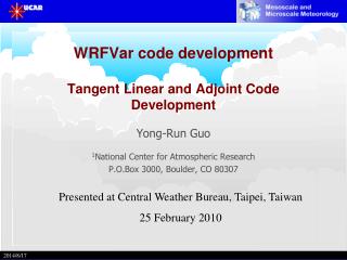
1. WRFVar code developmentTangent Linear and Adjoint Code Development Yong-Run Guo 1National Center for Atmospheric Research P.O.Box 3000, Boulder, CO 80307 Presented at Central Weather Bureau, Taipei, Taiwan 25 February 2010 2014/8/17

2. Introduction

3. Why do we have this talk about the adjoint code development manually? • To develop the adjoint of the model • Already done in MPG/MMM/NCAR for MM5 and WRF • To develop the adjoint of the observation operators • Must be done by users themselves • About the automatic tangent linear and adjoint generators

4. Formulation Cost function: Gradient, of with respect to the control variable x’ Forcing term to adjoint model:

5. Description of the variables • is a vector of the control variable, at t=0, and • is the non-linear model operator at time • is the perturbation vector of the control variable • C is the spatial interpolation operator • is the observation operator • is a observation vector • is the observation error covariance matrix. • The superscript means the tangent linear operator, and the superscript is the transpose or adjoint operator.

6. Availabe Automatical Tangent and Adjoint generators: TAF --- Transformation of Algorithms in Fortran http://www.autodiff.org/?module=Tools&tool=TAF TAPENADE http://www.autodiff.org/?module=Tools&tool=TAPENADE TAMC --- Tangent linear and Adjoint Model Compiler http://autodiff.com/tamc • Still few manual work needed: • Assign the independent input variables and the output variables; • Check the correctness of tangent linear and adjoint code; • Need the manually review, etc. • Do not fully understand the physical meaning and the logic of the code.

7. References Navon, L. M., X. Zou, J. Derber, and J. Sela, 1992: Variational data assimilation with an adiabatic version of the NMC spectral model. Mon. Wea. Rev.,120.1433-1446. Guo, Y.-R., Y.-H. Kuo, J. Dudhia, D. Parsons, and C. Rocken, 2000: Four-dimensional variational data assimilation of heterogeneous mesoscale observations for a strong convective case. Mon. Wea. Rev., 128, 619-643. Huang, X.-Y., et al.,2009: Four-dimensional variational data assimilation for WRF: Formulation and preliminary results. Mon. Wea. Rev., 137, 299-314. MM5 4DVAR code and documentation ftp://ftp.ucar.edu/mesouser/MM5_ADJ

8. During the forward model integration, compute and save the term from , , C, and : where and are from the observed data. In addition, users should also develop the code of C and N, and insert the calculations of the above forcing term and cost function in the subroutines. In WRFVar, the 2D and 3D spatial interpolation C and their adjoint code has already developed and located in WRFDA/var/da/da_interpolation. N should be developed if users want to assimilate a new type of observations.

9. In WRFVar, the incremental approach is used. For example, the ZTD operator is located in WRFDA/var/da/da_physics, the d(tr) and are located in WRFDA/var/da/da_gpspw.

10. Transformation from control variables V to the increment of the analysis variables: must be completed first: This transformation is completed in the directory: /WRFDA/var/da/da_vtox_transform. Note that the background error covariance matrix B is only appeared here. Cost function: Gradient, of with respect to the control variable V

11. During the adjoint model integration, compute and add the forcing term FC to adjoint model: where fc was mentioned above, but the adjoint code of and should be developed by users. In order to develop the adjoint code, the tangent linear code should be developed first.

12. Summary of WRFDA code • The core part of the WRFVar codes: • var/da/da_physics: Observation operators • var/da/_da_{obs-type}: Innovation and residuals • var/da/da_vtox_transform: transformation by using BE • var/da/da_minimization: Conjugate Gradient (CG)

13. Tangent Linear coding

14. Tangent linear code development ( see Tech. Note NCAR/TN-435-STR, 71-78, and 59) • The tangent linear operator is the first order approximation of the non-linear operator. The Taylor expansion where z is a vector of control variable, and z’ is a vector of the perturbation of control variable.is a Jacobian matrix. So the tangent linear operator is valid only when the z’ is very small, and the higher (than the second) order derivatives are very small.

15. To identify the independent variables and their functions, the constant variables in a Fortran code

16. Where are basic variables, are the perturbations, are the first derivatives. A, B, C, D are constants here. Note that there are no constants appearing in the tangent linear equations because the constants can never be perturbed.

17. Keep the values of the basic state exactly the same as those in the non-linear forward operator (model) because that is the starting point of the linearization in developing the tangent linear operator (model). In a practical application, to save the disk space to store the basic state, one may use some kind of approximation of the basic state (such as time-averaging values over certain intervals, or time-interpolation during the interval). But before doing that, the validation check of the tangent linear code must be done to guarantee that the results are making sense.

18. Correctness (or tangent linear validation) check From Taylor expansion, set , we can obtain Where is a parameter, and is a constant vector. When is small enough, but larger than the machine accuracy, the values of should be very close to 1.0 if the tangent linear code is correct. If the values of is not close to 1.0 with small , the tangent linear code is incorrect (or invalid). In the correctness check, the Fortran compiler must be with the option –r8.

19. Although the tangent linear operator is not used in the minimization process in a full, not incremental, 4DVAR system, the adjoint of the observation operator is developed based on the tangent linear operator (the first order approximation of the non-linear operator). So, the correctness of the tangent linear code must be guaranteed in developing the adjoint code. In increment 3DVAR, the tangent linear operator will be used as the forward observation operator.

20. Example: dew point TD The observation operator N for TD is And when TD > T, TD = T. Where the T, p, q are temperature, pressure and specific humidity. S1, S2, S3 are constants. Fortran code for TD: subroutine TQTD Input variable: T, P, Q Output variable: TD

21. SUBROUTINE TQTD(T,TD,P,Q) and when TD > T, TD = T.

22. Tangent linear code of TD Input variable: T, P, Q Basic state: T9, P9, Q9 Output variable: TD

23. Exercise: (i) relative humidity --- p (cb), T (k), and q (kg/kg) where Note: the units for temperature, specific humidity, and pressue are C, kg/kg, and Pa, respectively. The subroutines are located in WRFDA/var/da/da_physics: da_tp_to_qs.inc da_tp_to_qs_lin1.inc da_tp_to_qs_adj1.inc da_tpq_to_rh.inc da_tpq_to_rh_lin1.inc A Fortran program:RH.f90 for the tangent linear accuracy check. The results are in the next slide.

24. FORTRAN STOPZ0: t,p,q,es,qs,rh: 0.29000E+03 0.10000E+06 0.10000E-01 0.19180E+04 0.12012E-01 0.83248E+02Tangent linear Check for qs ================ 1 alpha=0.020 qs, qs0, dqs: 0.120881E-01 0.120123E-01 0.377992E-02 accu.=0.100278457E+01 2 alpha=0.040 qs, qs0, dqs: 0.121643E-01 0.120123E-01 0.377992E-02 accu.=0.100557812E+01 3 alpha=0.060 qs, qs0, dqs: 0.122410E-01 0.120123E-01 0.377992E-02 accu.=0.100838067E+01 4 alpha=0.080 qs, qs0, dqs: 0.123181E-01 0.120123E-01 0.377992E-02 accu.=0.101119225E+01 5 alpha=0.100 qs, qs0, dqs: 0.123956E-01 0.120123E-01 0.377992E-02 accu.=0.101401289E+01 6 alpha=0.120 qs, qs0, dqs: 0.124735E-01 0.120123E-01 0.377992E-02 accu.=0.101684263E+01 7 alpha=0.140 qs, qs0, dqs: 0.125519E-01 0.120123E-01 0.377992E-02 accu.=0.101968148E+01 8 alpha=0.160 qs, qs0, dqs: 0.126307E-01 0.120123E-01 0.377992E-02 accu.=0.102252947E+01 9 alpha=0.180 qs, qs0, dqs: 0.127100E-01 0.120123E-01 0.377992E-02 accu.=0.102538664E+01 10 alpha=0.200 qs, qs0, dqs: 0.127896E-01 0.120123E-01 0.377992E-02 accu.=0.102825302E+01 11 alpha=0.220 qs, qs0, dqs: 0.128698E-01 0.120123E-01 0.377992E-02 accu.=0.103112863E+01 12 alpha=0.240 qs, qs0, dqs: 0.129503E-01 0.120123E-01 0.377992E-02 accu.=0.103401349E+01 13 alpha=0.260 qs, qs0, dqs: 0.130314E-01 0.120123E-01 0.377992E-02 accu.=0.103690765E+01 14 alpha=0.280 qs, qs0, dqs: 0.131128E-01 0.120123E-01 0.377992E-02 accu.=0.103981113E+01 15 alpha=0.300 qs, qs0, dqs: 0.131947E-01 0.120123E-01 0.377992E-02 accu.=0.104272395E+01 16 alpha=0.320 qs, qs0, dqs: 0.132771E-01 0.120123E-01 0.377992E-02 accu.=0.104564616E+01 17 alpha=0.340 qs, qs0, dqs: 0.133599E-01 0.120123E-01 0.377992E-02 accu.=0.104857777E+01 18 alpha=0.360 qs, qs0, dqs: 0.134432E-01 0.120123E-01 0.377992E-02 accu.=0.105151881E+01 19 alpha=0.380 qs, qs0, dqs: 0.135269E-01 0.120123E-01 0.377992E-02 accu.=0.105446932E+01 20 alpha=0.400 qs, qs0, dqs: 0.136111E-01 0.120123E-01 0.377992E-02 accu.=0.105742933E+01Tangent linear Check for rh ================ 1 alpha=0.020 rh, rh0, drh: 0.830568E+02 0.832480E+02 -0.954611E+01 accu.=0.100132192E+01 2 alpha=0.040 rh, rh0, drh: 0.828651E+02 0.832480E+02 -0.954611E+01 accu.=0.100261687E+01 3 alpha=0.060 rh, rh0, drh: 0.826730E+02 0.832480E+02 -0.954611E+01 accu.=0.100388514E+01 4 alpha=0.080 rh, rh0, drh: 0.824804E+02 0.832480E+02 -0.954611E+01 accu.=0.100512699E+01 5 alpha=0.100 rh, rh0, drh: 0.822873E+02 0.832480E+02 -0.954611E+01 accu.=0.100634271E+01 6 alpha=0.120 rh, rh0, drh: 0.820938E+02 0.832480E+02 -0.954611E+01 accu.=0.100753255E+01 7 alpha=0.140 rh, rh0, drh: 0.818999E+02 0.832480E+02 -0.954611E+01 accu.=0.100869678E+01 8 alpha=0.160 rh, rh0, drh: 0.817056E+02 0.832480E+02 -0.954611E+01 accu.=0.100983568E+01 9 alpha=0.180 rh, rh0, drh: 0.815109E+02 0.832480E+02 -0.954611E+01 accu.=0.101094950E+01 10 alpha=0.200 rh, rh0, drh: 0.813158E+02 0.832480E+02 -0.954611E+01 accu.=0.101203851E+01 11 alpha=0.220 rh, rh0, drh: 0.811203E+02 0.832480E+02 -0.954611E+01 accu.=0.101310295E+01 12 alpha=0.240 rh, rh0, drh: 0.809245E+02 0.832480E+02 -0.954611E+01 accu.=0.101414309E+01 13 alpha=0.260 rh, rh0, drh: 0.807284E+02 0.832480E+02 -0.954611E+01 accu.=0.101515917E+01 14 alpha=0.280 rh, rh0, drh: 0.805319E+02 0.832480E+02 -0.954611E+01 accu.=0.101615145E+01 15 alpha=0.300 rh, rh0, drh: 0.803351E+02 0.832480E+02 -0.954611E+01 accu.=0.101712017E+01 16 alpha=0.320 rh, rh0, drh: 0.801381E+02 0.832480E+02 -0.954611E+01 accu.=0.101806558E+01 17 alpha=0.340 rh, rh0, drh: 0.799407E+02 0.832480E+02 -0.954611E+01 accu.=0.101898793E+01 18 alpha=0.360 rh, rh0, drh: 0.797430E+02 0.832480E+02 -0.954611E+01 accu.=0.101988744E+01 19 alpha=0.380 rh, rh0, drh: 0.795451E+02 0.832480E+02 -0.954611E+01 accu.=0.102076436E+01 20 alpha=0.400 rh, rh0, drh: 0.793470E+02 0.832480E+02 -0.954611E+01 accu.=0.102161892E+01

25. (ii) precipitable water --- accurate formula Assuming that the model has KX layers in vertical, and the heights of surface and model top, , , and the thickness of the layers, are known.

26. Adjoint coding

27. Adjoint code development (see Tech. Note NCAR/TN-435-STR, 79-99, and 59-60) Adjoint matrix is a transpose of the TLM matrix. The basic rule in writing the adjoint code from a tangent linear code is called the “Reverse rule”: In a Fortran statement, each of the left-side perturbation variable is moved to the right-side, and place the right-side variable in the position of this perturbation variable, with no change of its coefficient, to form each of the Fortran statements. One statement in the tangent linear code may become several statements in the adjoint code.

28. The Fortran statement of the tangent linear: The corresponding Fortran code of its adjoint:

29. In a segment of Fortran code (a series of statements in sub-routines, or main program), The last statement in the tangent linear code corresponds to the first statement in the adjoint code, and the first statement in the tangent linear code corresponds to the last statement in the adjoint code. The output variables from tangent linear code become the input variables to the adjoint code.

30. Basic 1 Statement 1 Basic 2 Statement 2 …………….. Basic N Statement N Tangent linear code Adjoint code Basic N Statement N(i) …………….. Basic 2 Statement 2(i) Basic 1 Statement 1(i) The following example clearly shows that the “reverse rule” is equivalent to the transpose of the matrix.

31. j i adjoint: forward: i j subroutine fwd(x,y,a,n,m) ! integer :: i, j, n, m real, dimension(1:m) :: x real, dimension(1:n) :: y real, dimension(n,m) :: a ! y = 0.0 ! do i = 1,n ! Fortran 77: ! do j = 1,m ! y(i) = a(i,j)*x(j) + y(i) ! enddo ! Fortran 90: y(i) = sum(a(i,:)*x(:)) enddo ! end subroutine fwd subroutine a_fwd(x,y,a,n,m) ! integer :: i, j, n, m real, dimension(1:m) :: x real, dimension(1:n) :: y real, dimension(n,m) :: a ! x = 0.0 ! do j = 1,m ! Fortran 77: ! do i = 1,n ! x(j) = a(i,j)*y(i) + x(j) ! enddo ! Fortran 90: x(j) = sum(a(:,j)*y(:)) enddo ! end subroutine a_fwd

32. To count the contributions from the input variables in the tangent linear code correctly ‘reuse’ problem --- All the contributions from an input variable in the TLM should be counted in the adjoint code, neither less nor more feedback to that TLM input variable. For example, Tangent linear code Here dx used twice. Adjoint code

33. ‘re-defined’ problem --- Do not mix the feedback in the adjoint code when the input variables were re-defined in TLM. Tangent linear code (redundant) Here dy is redefined. Adjoint code Not need these lines of code

34. * Re-calculate the basic state to guarantee it is exactly the same as that in the tangent linear model at the same point in the code sequence. This means that coefficients in the statements must be exactly the same in both tangent linear and its adjoint code.

35. Correctness check where is the arbitrary perturbation vector, is the tangent linear operator, and is the adjoint operator. Note: There is no approximation from TLM to Adjoint, the correctness check must have ’13-digit same’ accuracy for 64-bit data (with the compiler option –r8). Otherwise, the adjoint code is wrong.

36. ! program adj_check integer, parameter :: n = 3, m = 6 integer :: i, j real :: Righy, Left real, dimension(1:m) :: x0, x real, dimension(1:n) :: y real, dimension(n,m) :: a ! Initialize x: do j = 1,m x(j) = sin((3.14156/180.)*float(j-1)*15.) ! To keep a copy of x: x0(j) = x(j) ! Matrix a: do i = 1,n a(i,j) = 5.25*float(i) + float(j) enddo enddo ! print 10, ((a(i,j),j=1,m),i=1,n) 10 format('Matrix:a:'/(6f8.2)) print 11, (x (j),j=1,m) 11 format('input vector x :'/6e15.5) 12 format('input vector x0:'/6e15.5) !======================================= ! Forward: call fwd(x,y,a,n,m) ! Adjoint: call a_fwd(x,y,a,n,m) !======================================= ! ! ! Right = sum(y*y) ! ! ! print 11, (x (j),j=1,m) ! print 12, (x0(j),j=1,m) ! ! Left = sum(x0*x) ! print 20, Right, Left 20 format(/'Adjoint check:'/ & 10x,' Right=',E20.14/ & 10x,' Left =',E20.14)

37. Remember to have compiler option –r8, i.e. in Linux/PGI, pgf90 –r8 adj_check.f90 –o adj_check.exe adj_check.exe FORTRAN STOP Matrix:a: 6.25 7.25 8.25 9.25 10.25 11.25 11.50 12.50 13.50 14.50 15.50 16.50 16.75 17.75 18.75 19.75 20.75 21.75 input vector x : 0.00000E+00 0.25882E+00 0.50000E+00 0.70710E+00 0.86602E+00 0.96592E+00 Adjoint check: Right=0.79797532647807E+04 Left =0.79797532647807E+04

38. Examples: • precipitable water PW • The observation operator N for PW is Where the control variable q(k) is the specific humidity At k. , and is the acceleration of gravity. In this case, N = N’ because the observation operator is linear.

39. Adjoint code of PW: Fortran code for PW: subroutine PWATER: Input variable: PW Output variable: QVA Input variable: QVA Output variable: PW

40. Tangent linear code of TD Adjoint code of TD Input variable: T, P, Q Basic state: T9, P9, Q9 Output variable: TD

41. Exercise: • Can you point out which variables are re-used or re-defined in subroutine LTQTD (ATQTD)? • Write the adjoint code for relative humidity. • Write the adjoint code for accurate formula of precipitable water.