Assimilation Algorithms: Tangent Linear and Adjoint models
450 likes | 742 Vues
Assimilation Algorithms: Tangent Linear and Adjoint models. Yannick Trémolet ECMWF Data Assimilation Training Course March 2006. Introduction. 4D-Var is based on minimization algorithms: Conjugate Gradient, Newton methods (quasi-Newton, truncated…).

Assimilation Algorithms: Tangent Linear and Adjoint models
E N D
Presentation Transcript
Assimilation Algorithms:Tangent Linear and Adjoint models Yannick Trémolet ECMWF Data Assimilation Training Course March 2006
Introduction • 4D-Var is based on minimization algorithms: • Conjugate Gradient, • Newton methods (quasi-Newton, truncated…). • The cost function and its gradient are needed. • Overview: • Writing tangent linear and adjoint models, • Diagnostics.
4D Variational Assimilation • Model: • Observations: • Background: • Observation operator: • Cost function to minimise: • At the minimum
4D Variational Assimilation • Discretisation: • Observations: • Model: • Observation operator: • The cost function becomes:
Linearisation In the first order approximation, a perturbation of the control variable (initial condition) evolves acccording to the tangent linear model: The perturbation of the cost function is: Where is the linearised version of about , and are the departures from observations.
Linearisation And the gradient is given by:
Adjoint Equation We choose solution of the adjoint system: Then, we can show that: (Multiply by and sum over ). The gradientof the cost function is obtained by a backward integration of the adjoint model.
4D-Var Algorithm • Integrate forward model gives . • Integrate adjoint model backwards gives . • If STOP. • Compute descent direction (Newton, CG, …). • Compute step size : • Update initial condition:
Example: the Lorenz model Where is the time, the Prandtl number, the Rayleigh number, the aspect ratio, the intensity of convection, the maximum temperature difference and the stratification change due to convection (see references).
Lorenz model code SUBROUTINE model(x,dt,nstep) DO i=1,nstep CALL lorenz(x,dxdt) CALL step(x,dxdt,dt) ENDDO END SUBROUTINE model ! --------------------------- SUBROUTINE lorenz(x,dxdt) dxdt(1)=-p*x(1)+p*x(2) dxdt(2)=x(1)*(r-x(3))-x(2) dxdt(3)=x(1)*x(2)-b*x(3) END SUBROUTINE lorenz ! --------------------------- SUBROUTINE step(x,dxdt,dt) DO i=1,3 x(i)=x(i)+dt*dxdt(i) ENDDO END SUBROUTINE step
The linear code Linearise each line of the code one by one: dxdt(1) =-p*x(1) +p*x(2) -> dxdt_tl(1)=-p*x_tl(1)+p*x_tl(2) dxdt(2) = x(1)*(r-x(3)) -x(2) -> dxdt_tl(2)=x_tl(1)*(r-x(3)) -x(1)*x_tl(3) -x_tl(2) These can also be written as: dxdt(1)=-p*x(1)+p*x(2) dxdt(2)=x(1)*(r-xtraj(3))-xtraj(1)*x(3)-x(2) This writing convention can save a lot of typing... and errors !
Trajectory • The trajectory has to be available. It can be: • saved which costs memory, • recomputed which costs CPU time. • Intermediate options exist using checkpointing methods.
The tangent linear code SUBROUTINE model_tl(x,dt,nstep) DO i=1,nstep CALL get_trajectory(xtraj,i) CALL lorenz_tl(x,dxdt,xtraj) CALL step_tl(x,dxdt,dt) ENDDO END SUBROUTINE model_tl ! --------------------------- SUBROUTINE lorenz_tl(x,dxdt,xtraj) dxdt(1)=-p*x(1)+p*x(2) dxdt(2)=x(1)*(r-xtraj(3))-xtraj(1)*x(3)-x(2) dxdt(3)=x(1)*xtraj(2)+xtraj(1)*x(2)-b*x(3) END SUBROUTINE lorenz_tl ! --------------------------- SUBROUTINE step_tl(x,dxdt,dt) DO i=1,3 x(i)=x(i)+dt*dxdt(i) ENDDO END SUBROUTINE step_tl
Adjoint of one instruction From the tangent linear code: dxdt(1)=-p*x(1)+p*x(2) In matrix form, it can be written as: which can easily be transposed: The corresponding code is: x(1)=x(1)-p*dxdt(1) x(2)=x(2)+p*dxdt(1) dxdt(1)=0.
Adjoint of one instruction From the tangent linear code: dxdt(2)=x(1)*(r-xtraj(3))-xtraj(1)*x(3)-x(2) The adjoint is: x(1)=x(1)+(r-xtraj(3))*dxdt(2) x(2)=x(2)-dxdt(2) x(3)=x(3)-xtraj(1)*dxdt(2) dxdt(2)=0. Here again, the trajectory is needed.
The Adjoint Code Property of adjoints (transposition): Application: where represents the line of the tangent linear model. The adjoint code is made of the transpose of each line of the tangent linear code in reverse order.
Adjoint of loops In the TL code we had: DO i=1,3 x(i)=x(i)+dt*dxdt(i) ENDDO which is equivalent to x(1)=x(1)+dt*dxdt(1) x(2)=x(2)+dt*dxdt(2) x(3)=x(3)+dt*dxdt(3) We can reverse the order and transpose the lines: dxdt(3)=dxdt(3)+dt*x(3) dxdt(2)=dxdt(2)+dt*x(2) dxdt(1)=dxdt(1)+dt*x(1) which is equivalent to DO i=3,1,-1 dxdt(i)=dxdt(i)+dt*x(i) ENDDO
Conditional statements • What we want is the adjoint of the statements which were actually executed in the direct model. • We need to know which branch was executed • The result of the conditional has to be stored: it is part of the trajectory !!!
Remarks about adjoints • The adjoint always exists and it is unique, assuming spaces of finite dimension. Hence, coding the adjoint does not raise questions about its existence, only questions of technical implementation. • In the meteorological literature, the term adjoint is often improperly used to denote the adjoint of the tangent linear of a non-linear operator. One must be aware that discussions about the existence of the adjoint usually address the existence of the tangent linear model. • Without recomputation, the cost of the TL is usually about 1.5 times that of the non-linear code, the cost of the adjoint between 2 and 3 times that. • The tangent linear model is not necessary to run 4D-Var. It is needed as an intermediate step to write the adjoint.
Automatic differentiation • Writing the adjoint of a full meteorological model is a very long and very tedious process. • Existing tools: TAF (TAMC), TAPENADE (Odyssée), ... • Reverse the order of instructions, • Transpose instructions instantly without typos !!! • There are still unresolved issues: • It is NOT a black box tool, • Cannot handle non-differentiable instructions (TL is wrong), • Can create huge arrays to store the trajectory, • The code needs to be cleaned-up and optimised.
Use of Tangent Linear and Adjoint Models In Data Assimilation At ECMWF
Incremental 4D-VAR where : • computed at The cost function can be computed by integrating the tangent linear model.
Incremental 4D-VAR • Quadratic cost function allows for more efficient minimisation. • Because of the computational cost, the tangent linear and adjoint models are run at lower resolution. • The trajectory comes from a low resolution non-linear forecast. • Departures from observations are updated at high resolution twice (outer loop).
How accurate are our Tangent Linear and Adjoint Models ?
Diagnostics • Testing the linear and adjoint models. • Is the linear approximation valid in our 4D-VAR ? • Can we extend the 4D-VAR window ? • Can we increase the inner-loop resolution ? • Can we assimilate new weather parameters (rain, clouds…) ? • Can we evaluate algorithm changes ?
TL testing • Test of linear model based on Taylor series: • Valid for any perturbation (in practice a set of random vectors). • TL and NL run with the same setup: • Resolution • Physics • Time step • Simpler dynamics • Configuration (IFS)
The real world • In 4D-VAR the perturbation is not any vector, it is an analysis increment. It is not random and it is the result of a algorithm which involves the linear model. • The linear and non-linear models are used at different resolutions (T511/T159). • The non-linear model uses more physics. • Humidity is represented in spectral space in the linear model, in grid point space in the non-linear model.
Incremental test • Compare TL output with finite difference in 4D-VAR setup (resolution, physics, …). • All the necessary information is present during the minimisation: • High resolution non-linear update • Low resolution non-linear trajectory • Low resolution TL (cost function) • Minimisation (TL) • Low resolution TL (diagnostic) • High resolution non-linear update • All the components are used exactly in their 4D-VAR configuration.
Incremental test We can compute the relative error from 4D-Var output: Where is the pseudo-inverse of the simplification operator used in 4D-Var.
IFS: First minimisation • Relative error TL/finite diff. • Operational configuration, • T511/T159, • No TL physics.
IFS: Second minimisation • Operational configuration, • T511/T159, • With linear physics.
Time evolution of the error • T511/T159, • With physics.
Time evolution of the error (adiab.) • T511/T159, • No physics.
Impact of TL resolution (adiabatic) • T511 non linear, • No physics.
Impact of TL resolution • T511 non linear, • TL physics.
Impact of the TL physics • T511/T159, • 12h, • Adiabatic case represents the “upper bound”.
Longer 4D-VAR window • T511/T159, • 24h forecast. • It is not much worse than 12h!
Concluding remarks… • Diagnostics which cannot be carried out with the traditional test are possible: • Vertical interpolation, • Impact of resolution. • Does not replace the usual validation test. • 4D-VAR is tested, not just the TL model.
Concluding remarks… • Errors seem very large but 4D-VAR works !!! • The resolution of the inner loop has reached a limit with the current IFS linear model. • Better TL physics is needed (humidity, new data). • Adiabatic tests at T255 show that there is room for improvement.
Is there something wrong ? 2nd minimisation should be better (physics). 41
References • X. Y. Huang and X. Yang. Variational data assimilation with the Lorenz model. Technical Report 26, HIRLAM, April 1996. • E. Lorenz. Deterministic nonperiodic flow. J. Atmos. Sci., 20:130-141, 1963.