Efficient Sparse Direct Solvers on High-Performance Computers
This review explores sparse Gaussian elimination (GE) for solving systems of linear equations efficiently on high-performance computers. Topics include sparse structures, pivoting strategies, algorithmic issues, numerical stability, sparse factorization, and ordering techniques. The discussion covers the trade-offs between numerical accuracy and efficiency in sparse factorizations, highlighting methods such as static pivoting and numerical algorithms. Placement and control of fill-ins, optimal ordering for sparsity preservation, and practical considerations for implementing sparse solvers are crucial for maximizing performance and accuracy. Various algorithms and approaches, such as Nested Dissection Ordering and Weighted Bipartite Matching for static pivoting, are discussed in the context of achieving numerical accuracy while leveraging the benefits of parallelism in sparse solvers.

Efficient Sparse Direct Solvers on High-Performance Computers
E N D
Presentation Transcript
Sparse Direct Solvers on High Performance Computers X. Sherry Li xsli@lbl.gov http://crd.lbl.gov/~xiaoye CS267: Applications of Parallel Computers March 2, 2005
Review of Gaussian Elimination (GE) • Solving a system of linear equations Ax = b • First step of GE: • Repeats GE on C • Results in LU factorization (A = LU) • L lower triangular with unit diagonal, U upper triangular • Then x is obtained by solving two triangular systems with L and U
Sparse GE • Sparse systems are ubiquitous in science and engineering • Example: A of dimension 105,only 10~100 nonzeros per row • Goal: Store only nonzeros and perform operations only on nonzeros • Fill-in: original zero entry aijbecomes nonzero in L and U Natural order: nonzeros = 233Min. Degree order: nonzeros = 207
Numerical Stability: Need for Pivoting • One step of GE: • If α is small, some entries in B may be lost from addition • Pivoting: swap the current diagonal entry with a larger entry from the other part of the matrix • Goal: control element growth in L & U
Dense versus Sparse GE • Dense GE: Pr A Pc = LU • Pr and Pc are permutations chosen to maintain stability • Partial pivoting suffices in most cases : PrA = LU • Sparse GE: Pr A Pc = LU • Pr and Pc are chosen to maintain stability and preserve sparsity
Algorithmic Issues in Sparse GE • Minimize number of fill-ins, maximize parallelism • Sparsity structure of L & U depends on that of A, which can be changed by row/column permutations (vertex re-labeling of the underlying graph) • Ordering (combinatorial algorithms; NP-complete to find optimum [Yannakis ’83]; use heuristics) • Predict the fill-in positions in L & U • Symbolic factorization (combinatorial algorithms) • Design efficient data structure for storing and quick retrieval of the nonzeros • Compressed storage schemes • Perform factorization and triangular solutions • Numerical algorithms (F.P. operations only on nonzeros) • How and when to pivot ? • Usually dominate the total runtime
Numerical Pivoting • Goal of pivoting is to control element growth in L & U for stability • For sparse factorizations, often relax the pivoting rule to trade with better sparsity and parallelism (e.g., threshold pivoting, static pivoting , . . .) • Partial pivoting used in sequential SuperLU (GEPP) • Can force diagonal pivoting (controlled by diagonal threshold) • Hard to implement scalably for sparse factorization • Static pivoting used in SuperLU_DIST (GESP) • Before factor, scale and permute A to maximize diagonal: Pr Dr A Dc = A’ • Pr is found by a weighted bipartite matching algorithm on G(A) • During factor A’ = LU, replace tiny pivots by , without changing data structures for L & U • If needed, use a few steps of iterative refinement to improve the first solution • Quite stable in practice x s x b x x x
4 1 x x 3 x 4 5 2 2 2 1 3 3 4 4 5 5 5 3 Static Pivoting via Weighted Bipartite Matching G(A) A • Maximize the diag. entries: sum, or product (sum of logs) • Hungarian algo. or the like (MC64): O(n*(m+n)*log n) • Auction algo. (more parallel): O(n*m*log(n*C)) 1 1 row column
i i j k j k 1 1 i i Eliminate 1 j j k k • Undirected graph • After a vertex is eliminated, all its neighbors become a clique • The edges of the clique are the potential fills (upper bound !) 1 i i j j Eliminate 1 k k Structural Gaussian Elimination - Symmetric Case
Minimum Degree Ordering • Greedy approach: do the best locally • At each step • Eliminate the vertex with the smallest degree • Update degrees of the neighbors • Straightforward implementation is slow and requires too much memory • Newly added edges are more than eliminated vertices
Minimum Degree Ordering • Use quotient graph as a compact representation [George/Liu ’78] • Collection of cliques resulting from the eliminated vertices affects the degree of an uneliminated vertex • Represent each connected component in the eliminated subgraph by a single “supervertex” • Storage required to implement QG model is bounded by size of A • Large body of literature on implementation variations • Tinney/Walker `67, George/Liu `79, Liu `85, Amestoy/Davis/Duff `94, Ashcraft `95, Duff/Reid `95, et al., . . .
Nested Dissection Ordering • Global graph partitioning approach: top-down, divide-and-conquer • Nested dissection [George ’73, Lipton/Rose/Tarjan ’79] • First level • Recurse on A and B • Goal: find the smallest possible separator S at each level • Multilevel schemes [Hendrickson/Leland `94, Karypis/Kumar `95] • Spectral bisection [Simon et al. `90-`95] • Geometric and spectral bisection [Chan/Gilbert/Teng `94] A S B
Ordering for LU (unsymmetric) • Can use a symmetric ordering on a symmetrized matrix . . . • Case of partial pivoting (sequential SuperLU): Use ordering based on ATA • If RTR = ATA and PA = LU, then for any row permutation P, struct(L+U) struct(RT+R) [George/Ng `87] • Making R sparse tends to make L & U sparse . . . • Case of static pivoting (SuperLU_DIST): Use ordering based on AT+A • If RTR = AT+A and A = LU, then struct(L+U) struct(RT+R) • Making R sparse tends to make L & U sparse . . . • Can find better ordering based solely on A, without symmetrization [Amestoy/Li/Ng `03]
Ordering for Unsymmetric Matrix • Still wide open . . . • Simple extension: symmetric ordering using A’+A • Greedy algorithms, graph partitioning, or hybrid • Problem: unsymmetric structure is not respected ! • We developed an unsymmetric variant of “Min Degree” algorithm based solely on A [Amestoy/Li/Ng ’02] (a.k.a. Markowitz scheme)
c1 c2 c3 c1 c2 c3 1 1 r1 r1 Eliminate 1 Eliminate 1 r2 r2 • Bipartite graph • After a vertex is eliminated, all the row & column vertices adjacent to • it become fully connected – “bi-clique” (assuming diagonal pivot) • The edges of the bi-clique are the potential fills (upper bound!) r1 r1 1 c1 1 c1 c2 c2 r2 r2 c3 c3 Structural Gaussian Elimination - Unsymmetric Case
Results of Markowitz Ordering • Extend the QG model to bipartite quotient graph • Same asymptotic complexity as symmetric MD • Space is bounded by 2*(m + n) • Time is bounded by O(n * m) • For 50+ unsym. matrices, compared with MD on A’+A: • Reduction in fill: average 0.88, best 0.38 • Reduction in f.p. operations: average0.77, best 0.01 • How about graph partitioning? • Use directed graph
Techniques to Reduce Memory Access & Communication Cost • Blocking to increase number of floating-point operations performed for each memory access • Aggregate small messages into one larger message • Reduce cost due to latency • Well done in LAPACK, ScaLAPACK • Dense and banded matrices • Adopted in the new generation sparse software • Performance much more sensitive to latency in sparse case
Benefits of Supernodes: Permit use of Level 3 BLAS (e.g., matrix-matrix mult.) Reduce inefficient indirect addressing. Reduce symbolic time by traversing supernodal graph. Exploit dense submatrices in L & U factors Blocking in Sparse GE
Speedup Over Un-blocked Code • Matrices sorted in increasing #Flops/nonzeros • Up to 40% of machine peak on large sparse matrices on IBM RS6000/590, MIPS R8000, 25% on Alpha 21164
Parallel Task Scheduling for SMPs (in SuperLU_MT) • Elimination tree exhibits parallelism and dependencies Shared task queue initialized by leaves While ( there are more panels ) do panel := GetTask( queue ) (1) panel_symbolic_factor( panel ) • Skip all BUSY descendant supernodes (2) panel_numeric_factor( panel ) • Perform updates from all DONE supernodes • Wait for BUSY supernodes to become DONE (3) inner_factor( panel ) End while • Up to 25-30% machine peak, 20 processors, Cray C90/J90, SGI Origin
Parallelism from Separator Tree • Come from graph partitioning type of ordering
Matrix Distribution on Large Distributed-memory Machine • 2D block cyclic recommended for many linear algebra algorithms • Better load balance, less communication, and BLAS-3 1D blocked 1D cyclic 1D block cyclic 2D block cyclic
2D Block Cyclic Layout for Sparse L and U (in SuperLU_DIST) • Better for GE scalability, load balance
Scalability and Isoefficiency Analysis • Model problem: matrix from 11 pt Laplacian on k x k x k (3D) mesh; Nested dissection ordering • N = k3 • Factor nonzeros : O(N4/3) • Number of floating-point operations : O(N2) • Total communication overhead : O(N4/3 P) (assuming P processors arranged as grid) • Isoefficiency function: Maintain constant efficiency if Work increases proportionally with Overhead: This is equivalent to: • (Memory-processor relation) • Parallel efficiency can be kept constant if the memory-per-processor is constant, same as dense LU in ScaLPAPACK • (Work-processor relation)
Scalability • 3D KxKxK cubic grids, scale N2 = K6 with P for constant work per processor • Achieved 12.5 and 21.2 Gflops on 128 processors • Performance sensitive to communication latency • Cray T3E latency: 3 microseconds ( ~ 2702 flops) • IBM SP latency: 8 microseconds ( ~ 11940 flops )
Adoptions of SuperLU • Industrial • FEMLAB • HP Mathematical Library • Mathematica • NAG • Numerical Python • Academic/Lab: • In other ACTS Tools: PETSc, Hyper • M3D, NIMROD (simulate fusion reactor plasmas) • Omega3P (accelerator design, SLAC) • OpenSees (earthquake simluation, UCB) • DSpice (parallel circuit simulation, SNL) • Trilinos (object-oriented framework encompassing various solvers, SNL) • NIKE (finite element code for structural mechanics, LLNL)
Summary • Important kernel for science and engineering applications, used in practice on a regular basis • Good implementation on high-performance machines needa large set of tools from CS and NLA • Performance more sensitive to latency than dense case • Survey of other sparse direct solvers: “Eigentemplates” book http://crd.lbl.gov/~xiaoye/SuperLU/SparseDirectSurvey.pdf • LLT, LDLT, LU
Application 1: Quantum Mechanics • Scattering in a quantum system of three charged particles • Simplest example is ionization of a hydrogen atom by collision with an electron: e- + H H+ + 2e- • Seek the particles’ wave functions represented by the time-independent Schrodinger equation • First solution to this long-standing unsolved problem [Recigno, McCurdy, et al. Science, 24 Dec 1999]
Quantum Mechanics (cont.) • Finite difference leads to complex, unsymmetric systems, very ill-conditioned • Diagonal blocks have the structure of 2D finite difference Laplacian matrices Very sparse: nonzeros per row <= 13 • Off-diagonal block is a diagonal matrix • Between 6 to 24 blocks, each of order between 200K and 350K • Total dimension up to 8.4 M • Too much fill if use direct method . . .
SuperLU_DIST as Preconditioner • SuperLU_DIST as block-diagonal preconditioner for CGS iteration M-1A x = M-1b M = diag(A11, A22, A33, …) • Run multiple SuperLU_DIST simultaneously for diagonal blocks • No pivoting, nor iterative refinement • 12 to 35 CGS iterations @ 1 ~ 2 minute/iteration using 64 IBM SP processors • Total time: 0.5 to a few hours
Complex, unsymmetric N = 2 M, NNZ = 26 M Fill-ins using Metis: 1.3 G (50x fill) Factorization speed 10x speedup (4 to 128 P) Up to 30 Gflops One Block Timings on IBM SP
Application 2: Accelerator Cavity Design • Calculate cavity mode frequencies and field vectors • Solve Maxwell equation in electromagnetic field • Omega3P simulation code developed at SLAC Omega3P model of a 47-cell section of the 206-cell Next Linear Collider accelerator structure Individual cells used in accelerating structure
Finite element methods lead to large sparse generalized eigensystem K x = M x Real symmetric for lossless cavities; Complex symmetric when lossy in cavities Seek interior eigenvalues (tightly clustered) that are relatively small in magnitude Accelerator (cont.)
Accelerator (cont.) • Speed up Lanczos convergence by shift-invert Seek largest eigenvalues, well separated, of the transformed system M (K - M)-1 x = M x = 1 / ( - ) • The Filtering algorithm [Y. Sun] • Inexact shift-invert Lanczos + JOCC (Jacobi Orthogonal Component Correction) • We added exact shift-invert Lanczos (ESIL) • PARPACK for Lanczos • SuperLU_DIST for shifted linear system • No pivoting, nor iterative refinement
DDS47, Linear Elements • Total eigensolver time: N = 1.3 M, NNZ = 20 M
Largest Eigen Problem Solved So Far • DDS47, quadratic elements • N = 7.5 M, NNZ = 304 M • 6 G fill-ins using Metis • 24 processors (8x3) • Factor: 3,347 s • 1 Solve: 61 s • Eigensolver: 9,259 s (~2.5 hrs) • 10 eigenvalues, 1 shift, 55 solves


