Download
1 / 23
230 likes | 404 Vues
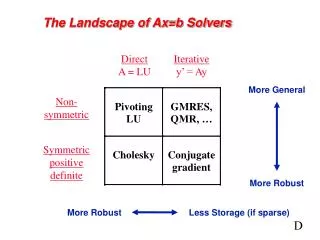
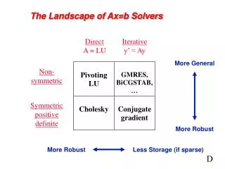
Direct A = LU. Iterative y ’ = Ay. More General. Non- symmetric. Symmetric positive definite. More Robust. More Robust. Less Storage. The Landscape of Sparse Ax=b Solvers. D. for j = 1 : n L( j:n , j) = A( j:n , j); for k = 1 : j-1 % cmod ( j,k )

E N D
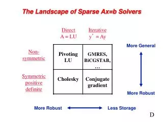
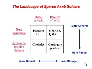
Direct A = LU Iterative y’ = Ay More General Non- symmetric Symmetric positive definite More Robust More Robust Less Storage The Landscape of Sparse Ax=b Solvers D
for j = 1 : n L(j:n, j) = A(j:n, j); for k = 1 : j-1 % cmod(j,k) L(j:n, j) = L(j:n, j) – L(j, k) * L(j:n, k); end; % cdiv(j) L(j, j) = sqrt(L(j, j)); L(j+1:n, j) = L(j+1:n, j) / L(j, j); end; j LT L A L Column Cholesky Factorization • Column j of A becomes column j of L
for j = 1 : n L(j:n, j) = A(j:n, j); for k < j with L(j, k) nonzero % sparse cmod(j,k) L(j:n, j) = L(j:n, j) – L(j, k) * L(j:n, k); end; % sparse cdiv(j) L(j, j) = sqrt(L(j, j)); L(j+1:n, j) = L(j+1:n, j) / L(j, j); end; j LT L A L Sparse Column Cholesky Factorization • Column j of A becomes column j of L
3 7 1 3 7 1 6 8 6 8 4 10 4 10 9 2 9 2 5 5 Graphs and Sparse Matrices: Cholesky factorization Fill:new nonzeros in factor Symmetric Gaussian elimination: for j = 1 to n add edges between j’s higher-numbered neighbors G+(A)[chordal] G(A)
Cholesky Graph Game Given an undirected graph G = G(A), Repeat: Choose a vertex v and mark it; Add edges between unmarked neighbors of v; Until every vertex is marked Goal: End up with as few edges as possible. Output: A labeling of the vertices with numbers 1 to n, corresponding to a symmetric permutation of matrix A.
Path lemma [Davis Thm 4.1] Let G = G(A) be the graph of a symmetric, positive definite matrix, with vertices 1, 2, …, n, and let G+ = G+(A)be the filled graph. Then (v, w) is an edge of G+if and only if G contains a path from v to w of the form (v, x1, x2, …, xk, w) with xi < min(v, w) for each i. (This includes the possibility k = 0, in which case (v, w) is an edge of G and therefore of G+.)
3 7 1 6 8 10 4 10 9 5 4 8 9 2 2 5 7 3 6 1 Elimination Tree G+(A) T(A) Cholesky factor • T(A) : parent(j) = min { i > j : (i, j) inG+(A) } • parent(col j) = first nonzero row below diagonal in L • T describes dependencies among columns of factor • Can compute G+(A) easily from T • Can compute T from G(A) in almost linear time
Facts about elimination trees • If G(A) is connected, then T(A) is connected (it’s a tree, not a forest). • If A(i, j) is nonzero and i > j, then i is an ancestor of j in T(A). • If L(i, j) is nonzero, then i is an ancestor of j in T(A). [Davis Thm 4.4] • T(A) is a depth-first spanning tree of G+(A). • T(A) is the transitive reduction of the directed graph G(LT).
Describing the nonzero structure of L in terms of G(A) and T(A) • If (i, k) is an edge of G with i > k, then the edges of G+ include: (i, k) ; (i, p(k)) ; (i, p(p(k))) ; (i, p(p(p(k)))) . . . • Let i > j. Then (i, j) is an edge of G+ iff j is an ancestor in T of some k such that (i, k) is an edge of G. • The nonzeros in row i of L are a “row subtree” of T. • The nonzeros in col j of L are some ofj’s ancestors in T. • Just the ones adjacent in G to vertices in the subtree of T rooted at j.
Symbolic factorization: Computing G+(A) T and G give the nonzero structure of L either by rows or by columns. • Row subtrees[Davis Fig 4.4]: Tr[i] is the subtree of T formed by the union of the tree paths from j to i, for all edges (i, j) of G with j < i. • Tr[i] is rooted at vertex i. • The vertices of Tr[i] are the nonzeros of row i of L. • For j < i, (i, j) is an edge of G+ iff j is a vertex of Tr[i]. • Column unions[Davis Fig 4.10]: Column structures merge up the tree. • struct(L(:, j)) = struct(A(j:n, j)) + union( struct(L(:,k)) | j = parent(k) in T ) • For i > j, (i, j) is an edge of G+ iff either (i, j) is an edge of G or (i, k) is an edge of G+ for some child k of j in T. • Running time is O(nnz(L)), which is best possible . . . • . . . unless we just want the nonzero counts of the rows and columns of L
Complexity measures for sparse Cholesky • Space: • Measured by fill, which is nnz(G+(A)) • Number of off-diagonal nonzeros in Choleskyfactor (need to store about n + nnz(G+(A)) real numbers). • Sum over vertices of G+(A) of (# of higher neighbors). • Time: • Measured by number of flops(multiplications, say) • Sum over vertices of G+(A) of (# of higher neighbors)2 • Front size: • Related to the amount of “fast memory” required • Max over vertices of G+(A) of (# of higher neighbors).
Permutations for sparsity “I observed that most of the coefficients in our matrices were zero; i.e., the nonzeros were ‘sparse’ in the matrix, and that typically the triangular matrices associated with the forward and back solution provided by Gaussian elimination would remain sparse if pivot elements were chosen with care” - Harry Markowitz, describing the 1950s work on portfolio theory that won the 1990 Nobel Prize for Economics
Cholesky Graph Game Given an undirected graph G = G(A), Repeat: Choose a vertex v and mark it; Add edges between unmarked neighbors of v; Until every vertex is marked Goal: End up with as few edges as possible. Output: A labeling of the vertices with numbers 1 to n, corresponding to a symmetric permutation of matrix A.
n1/2 The (2-dimensional) model problem • Graph is a regular square grid with n = k2vertices. • Corresponds to matrix for regular 2D finite difference mesh. • Gives good intuition for behavior of sparse matrix algorithms on many 2-dimensional physical problems. • There’s also a 3-dimensional model problem.
Permutations of the 2-D model problem • Theorem 1:With the natural permutation, the n-vertex model problem has exactly O(n3/2) fill. • Theorem 2:With a nested dissection permutation, the n-vertex model problem has exactly O(n log n) fill. • Theorem 3:With any permutation, the n-vertex model problem has at least O(n log n) fill. See course notes for proofs.
Nested dissection ordering • Aseparatorin a graph G is a set S of vertices whose removal leaves at least two connected components. • A nested dissection ordering for an n-vertex graph G numbers its vertices from 1 to n as follows: • Find a separator S, whose removal leaves connected components T1, T2, …, Tk • Number the vertices of S from n-|S|+1 to n. • Recursively, number the vertices of each component:T1 from 1 to |T1|, T2 from |T1|+1 to |T1|+|T2|, etc. • If a component is small enough, number it arbitrarily. • It all boils down to finding good separators!
Separators in theory • If G is a planar graph with n vertices, there exists a set of at most sqrt(6n) vertices whose removal leaves no connected component with more than 2n/3 vertices. (“Planar graphs have sqrt(n)-separators.”) • “Well-shaped” finite element meshes in 3 dimensions have n2/3 - separators. • Also some other classes of graphs – trees, graphs of bounded genus, chordal graphs, bounded-excluded-minor graphs, … • Mostly these theorems come with efficient algorithms, but they aren’t used much.
Separators in practice • Graph partitioning heuristics have been an active research area for many years, often motivated by partitioning for parallel computation. See CS 240A. • Some techniques: • Spectral partitioning (uses eigenvectors of Laplacian matrix of graph) • Geometric partitioning (for meshes with specified vertex coordinates) • Iterative-swapping (Kernighan-Lin, Fiduccia-Matheysses) • Breadth-first search (fast but dated) • Many popular modern codes (e.g. Metis, Chaco) use multilevel iterative swapping • Matlab graph partitioning toolbox: see course web page
Permutations of general 2D and 3D problems • Theorem 4:With a nested dissection permutation, any planar graph with n vertices has at most O(n log n) fill. • Theorem 5:With a nested dissection permutation, any 3D finite element mesh (with a technical condition on element shapes) has at most O(n 4/3 ) fill. See course notes for references to proofs.
Heuristic fill-reducing matrix permutations • Nested dissection: • Find a separator, number it last, proceed recursively • Theory: approx optimal separators => approx optimal fill and flop count • Practice: often wins for very large problems • Minimum degree: • Eliminate row/col with fewest nzs, add fill, repeat • Hard to implement efficiently – current champion is “Approximate Minimum Degree”[Amestoy, Davis, Duff] • Theory: can be suboptimal even on 2D model problem • Practice: often wins for medium-sized problems • Banded orderings (Reverse Cuthill-McKee, Sloan, . . .): • Try to keep all nonzeros close to the diagonal • Theory, practice: often wins for “long, thin” problems • The best modern general-purpose orderings are ND/MD hybrids.
Fill-reducing permutations in Matlab • Symmetric approximate minimum degree: • p = amd(A); • symmetric permutation: chol(A(p,p)) often sparser than chol(A) • Symmetric nested dissection: • not built into Matlab • several versions in meshpart toolbox (course web page references) • Nonsymmetric approximate minimum degree: • p = colamd(A); • column permutation: lu(A(:,p)) often sparser than lu(A) • also for QR factorization • Reverse Cuthill-McKee • p = symrcm(A); • A(p,p) often has smaller bandwidth than A • similar to Sparspak RCM
n1/2 n1/3 Complexity of direct methods Time and space to solve any problem on any well-shaped finite element mesh
Sparse Cholesky factorization to solve Ax = b • Preorder: replace A by PAPT and b by Pb • Independent of numerics • Symbolic Factorization: build static data structure • Elimination tree • Nonzero counts • Supernodes • Nonzero structure of L • Numeric Factorization: A = LLT • Static data structure • Supernodes use BLAS3 to reduce memory traffic • Triangular Solves: solve Ly = b, then LTx = y