CS 240A: Solving Ax = b in parallel

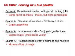
CS 240A: Solving Ax = b in parallel • Dense A: Gaussian elimination with partial pivoting (LU) • Same flavor as matrix * matrix, but more complicated • Sparse A: Gaussian elimination – Cholesky, LU, etc. • Graph algorithms • Sparse A: Iterative methods – Conjugate gradient, etc. • Sparse matrix times dense vector • Sparse A: Preconditioned iterative methods and multigrid • Mixture of lots of things

2 1 4 5 7 6 3 Matrix and Graph • Edge from row i to column j for nonzero A(i,j) • No edges for diagonal nonzeros • If A is symmetric, G(A) is an undirected graph • Symmetric permutation PAPTrenumbers the vertices A G(A)

Compressed Sparse Matrix Storage value: • Full storage: • 2-dimensional array. • (nrows*ncols) memory. row: colstart: • Sparse storage: • Compressed storage by columns (CSC). • Three 1-dimensional arrays. • (2*nzs + ncols + 1) memory. • Similarly,CSR.

Direct A = LU Iterative y’ = Ay More General Non- symmetric Symmetric positive definite More Robust The Landscape of Ax=b Solvers More Robust Less Storage (if sparse)

CS 240A: Solving Ax = b in parallel • Dense A: Gaussian elimination with partial pivoting (LU) • See April 15 slides • Same flavor as matrix * matrix, but more complicated • Sparse A: Gaussian elimination – Cholesky, LU, etc. • Graph algorithms • Sparse A: Iterative methods – Conjugate gradient, etc. • Sparse matrix times dense vector • Sparse A: Preconditioned iterative methods and multigrid • Mixture of lots of things

Gaussian elimination to solve Ax = b For a symmetric, positive definite matrix: • Matrix factorization: A = LLT (Cholesky factorization) • Forward triangular solve: Ly = b • Backward triangular solve: LTx = y For a nonsymmetric matrix: • Matrix factorization: PA = LU (Partial pivoting) • . . .

for j = 1 : n L(j:n, j) = A(j:n, j); for k < j with L(j, k) nonzero % sparse cmod(j,k) L(j:n, j) = L(j:n, j) – L(j, k) * L(j:n, k); end; % sparse cdiv(j) L(j, j) = sqrt(L(j, j)); L(j+1:n, j) = L(j+1:n, j) / L(j, j); end; j LT L A L Sparse Column Cholesky Factorization • Column j of A becomes column j of L

Irregular mesh: NASA Airfoil in 2D

3 7 1 3 7 1 6 8 6 8 4 10 4 10 9 2 9 2 5 5 Graphs and Sparse Matrices: Cholesky factorization Fill:new nonzeros in factor Symmetric Gaussian elimination: for j = 1 to n add edges between j’s higher-numbered neighbors G+(A)[chordal] G(A)

Permutations of the 2-D model problem • Theorem:With the natural permutation, the n-vertex model problem has (n3/2) fill. (“order exactly”) • Theorem:With any permutation, the n-vertex model problem has (n log n) fill. (“order at least”) • Theorem:With a nested dissection permutation, the n-vertex model problem has O(n log n) fill. (“order at most”)

Nested dissection ordering • Aseparatorin a graph G is a set S of vertices whose removal leaves at least two connected components. • A nested dissection ordering for an n-vertex graph G numbers its vertices from 1 to n as follows: • Find a separator S, whose removal leaves connected components T1, T2, …, Tk • Number the vertices of S from n-|S|+1 to n. • Recursively, number the vertices of each component:T1 from 1 to |T1|, T2 from |T1|+1 to |T1|+|T2|, etc. • If a component is small enough, number it arbitrarily. • It all boils down to finding good separators!

Separators in theory • If G is a planar graph with n vertices, there exists a set of at most sqrt(6n) vertices whose removal leaves no connected component with more than 2n/3 vertices. (“Planar graphs have sqrt(n)-separators.”) • “Well-shaped” finite element meshes in 3 dimensions have n2/3 - separators. • Also some other classes of graphs – trees, graphs of bounded genus, chordal graphs, bounded-excluded-minor graphs, … • Mostly these theorems come with efficient algorithms, but they aren’t used much.

Separators in practice • Graph partitioning heuristics have been an active research area for many years, often motivated by partitioning for parallel computation. • Some techniques: • Spectral partitioning (uses eigenvectors of Laplacian matrix of graph) • Geometric partitioning (for meshes with specified vertex coordinates) • Iterative-swapping (Kernighan-Lin, Fiduccia-Matheysses) • Breadth-first search (fast but dated) • Many popular modern codes (e.g. Metis, Chaco) use multilevel iterative swapping • Matlab graph partitioning toolbox: see course web page

n1/2 n1/3 Complexity of direct methods Time and space to solve any problem on any well-shaped finite element mesh

Direct A = LU Iterative y’ = Ay More General Non- symmetric Symmetric positive definite More Robust The Landscape of Ax=b Solvers More Robust Less Storage (if sparse)

Conjugate gradient iteration x0 = 0, r0 = b, d0 = r0 for k = 1, 2, 3, . . . αk = (rTk-1rk-1) / (dTk-1Adk-1) step length xk = xk-1 + αk dk-1 approx solution rk = rk-1 – αk Adk-1 residual βk = (rTk rk) / (rTk-1rk-1) improvement dk = rk + βk dk-1 search direction • One matrix-vector multiplication per iteration • Two vector dot products per iteration • Four n-vectors of working storage

Sparse matrix data structure (stored by rows) • Full: • 2-dimensional array of real or complex numbers • (nrows*ncols) memory • Sparse: • compressed row storage • about (2*nzs + nrows) memory

Distributed row sparse matrix data structure P0 P1 • Each processor stores: • # of local nonzeros • range of local rows • nonzeros in CSR form P2 Pp-1

P0 P1 P2 P3 x P0 P1 P2 P3 y Matrix-vector product: Parallel implementation • Lay out matrix and vectors by rows • y(i) = sum(A(i,j)*x(j)) • Skip terms with A(i,j) = 0 • Algorithm Each processor i: Broadcast x(i) Compute y(i) = A(i,:)*x • Optimizations: reduce communication by • Only send as much of x as necessary to each proc • Reorder matrix for better locality by graph partitioning

Sparse Matrix-Vector Multiplication

Conjugate gradient: Convergence • In exact arithmetic, CG converges in n steps (completely unrealistic!!) • Accuracy after k steps of CG is related to: • consider polynomials of degree k that are equal to 1 at 0. • how small can such a polynomial be at all the eigenvalues of A? • Thus, eigenvalues close together are good. • Condition number:κ(A) = ||A||2 ||A-1||2 = λmax(A) / λmin(A) • Residual is reduced by a constant factor by O( sqrt(κ(A)) ) iterations of CG.

Preconditioners • Suppose you had a matrix B such that: • condition number κ(B-1A) is small • By = z is easy to solve • Then you could solve (B-1A)x = B-1b instead of Ax = b • Each iteration of CG multiplies a vector by B-1A: • First multiply by A • Then solve a system with B

Preconditioned conjugate gradient iteration x0 = 0, r0 = b, d0 = B-1r0, y0 = B-1r0 for k = 1, 2, 3, . . . αk = (yTk-1rk-1) / (dTk-1Adk-1) step length xk = xk-1 + αk dk-1 approx solution rk = rk-1 – αk Adk-1 residual yk = B-1rk preconditioning solve βk = (yTk rk) / (yTk-1rk-1) improvement dk = yk + βk dk-1 search direction • One matrix-vector multiplication per iteration • One solve with preconditioner per iteration

Choosing a good preconditioner • Suppose you had a matrix B such that: • condition number κ(B-1A) is small • By = z is easy to solve • Then you could solve (B-1A)x = B-1b instead of Ax = b • B = A is great for (1), not for (2) • B = I is great for (2), not for (1) • Domain-specific approximations sometimes work • B = diagonal of A sometimes works • Better: blend in some direct-methods ideas. . .

x A RT R Incomplete Cholesky factorization (IC, ILU) • Compute factors of A by Gaussian elimination, but ignore fill • Preconditioner B = RTR  A, not formed explicitly • Compute B-1z by triangular solves (in time nnz(A)) • Total storage is O(nnz(A)), static data structure • Either symmetric (IC) or nonsymmetric (ILU)

1 4 1 4 3 2 3 2 Incomplete Cholesky and ILU: Variants • Allow one or more “levels of fill” • unpredictable storage requirements • Allow fill whose magnitude exceeds a “drop tolerance” • may get better approximate factors than levels of fill • unpredictable storage requirements • choice of tolerance is ad hoc • Partial pivoting (for nonsymmetric A) • “Modified ILU” (MIC): Add dropped fill to diagonal of U or R • A and RTR have same row sums • good in some PDE contexts

Incomplete Cholesky and ILU: Issues • Choice of parameters • good: smooth transition from iterative to direct methods • bad: very ad hoc, problem-dependent • tradeoff: time per iteration (more fill => more time)vs # of iterations (more fill => fewer iters) • Effectiveness • condition number usually improves (only) by constant factor (except MIC for some problems from PDEs) • still, often good when tuned for a particular class of problems • Parallelism • Triangular solves are not very parallel • Reordering for parallel triangular solve by graph coloring

Coloring for parallel nonsymmetric preconditioning [Aggarwal, Gibou, G] 263 million DOF • Level set method for multiphase interface problems in 3D • Nonsymmetric-structure, second-order-accurate octree discretization. • BiCGSTAB preconditioned by parallel triangular solves.

A B-1 Sparse approximate inverses • Compute B-1 A explicitly • Minimize || B-1A – I ||F (in parallel, by columns) • Variants: factored form of B-1, more fill, . . • Good: very parallel • Bad: effectiveness varies widely

Other Krylov subspace methods • Nonsymmetric linear systems: • GMRES: for i = 1, 2, 3, . . . find xi  Ki (A, b) such that ri= (Axi – b)  Ki (A, b)But, no short recurrence => save old vectors => lots more space (Usually “restarted” every k iterations to use less space.) • BiCGStab, QMR, etc.:Two spaces Ki (A, b) and Ki (AT, b) w/ mutually orthogonal basesShort recurrences => O(n) space, but less robust • Convergence and preconditioning more delicate than CG • Active area of current research • Eigenvalues: Lanczos (symmetric), Arnoldi (nonsymmetric)

Multigrid • For a PDE on a fine mesh, precondition using a solution on a coarser mesh • Use idea recursively on hierarchy of meshes • Solves the model problem (Poisson’s eqn) in linear time! • Often useful when hierarchy of meshes can be built • Hard to parallelize coarse meshes well • This is just the intuition – lots of theory and technology

n1/2 n1/3 Complexity of linear solvers Time to solve model problem (Poisson’s equation) on regular mesh

n1/2 n1/3 Complexity of direct methods Time and space to solve any problem on any well-shaped finite element mesh

CS 240A: Solving Ax = b in parallel