Download
1 / 40
400 likes | 624 Vues
NONLINEAR MAPPING: APPROACHES BASED ON OPTIMIZING AN INDEX OF CONTINUITY AND APPLYING CLASSICAL METRIC MDS TO REVISED DISTANCES By Ulas Akkucuk. & J. Douglas Carroll Rutgers Business School – Newark and New Brunswick. Outline. Introduction Nonlinear Mapping Algorithms

E N D
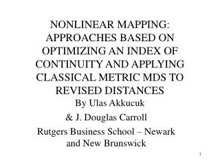
NONLINEAR MAPPING: APPROACHES BASED ON OPTIMIZING AN INDEX OF CONTINUITY AND APPLYING CLASSICAL METRIC MDS TO REVISED DISTANCESBy Ulas Akkucuk & J. Douglas Carroll Rutgers Business School – Newark and New Brunswick
Outline • Introduction • Nonlinear Mapping Algorithms • Parametric Mapping Approach • ISOMAP Approach • Other Approaches • Experimental Design and Methods • Error Levels • Evaluation of Mapping Performance • Problem of Similarity Transformations • Results • Discussion and Future Direction
Introduction • Problem: To determine a smaller set of variables necessary to account for a larger number of observed variables • PCA and MDS are useful when relationship is linear • Alternative approaches needed when the relationship is highly nonlinear
Shepard and Carroll (1966) • Locally monotone analysis of proximities: Nonmetric MDS treating large distances as missing • Worked well if the nonlinearities were not too severe (in particular if the surface is not closed such as a circle or sphere) • Optimization of an index of “continuity” or “smoothness” • Incorporated into a computer program called “PARAMAP” and tested on various sets of data
62 regularly spaced points on a sphere, and the azimuthal equidistant projection of the world
49 points regularly spaced on a torus embedded in four dimensions
In all cases the local structure is preserved except points at which the shape is “cut open” or “punctured” • Results were successful, but severe local minimum problem existed • Addition of error to the regular spacing made the local minimum problem worse • Current work is stimulated by two articles on nonlinear mapping (Tenenbaum, de Silva, & Langford, 2000; Roweis & Saul, 2000)
Nonlinear Mapping Algorithms • n : number of objects • M : dimensionality of the input coordinates, in other words of the configuration for which we would like to find an underlying lower dimensional embedding. • R : dimensionality of the space of recovered configuration, where R<M • Y : n M input matrix • X : n R output matrix
The distances between point i and point j in the input and output spaces respectively are calculated as: [ ij ] D [ dij ]
Parametric Mapping Approach • Works via optimizing an index of “continuity” or “smoothness” • Early application in the context of time-series data (von Neuman, Kent, Bellison, & Hart, 1941; von Neuman, 1941)
A more general expression for the numerator is: • Generalizing to the multidimensional case we reach
Several modifications needed for the minimization procedure: • d2ij + Ce2 is substituted for d2ij , C is a constant equal to 2 / (n - 1) and e takes on values between 0 and 1 • e has a practical effect on accelerating the numerical process • Can be thought of as an extra “specific” dimension, as e gets closer to 0 points are made to approach “common” part of space
In the numerator the constant z, and in the denominator [2/n(n1)]2 • Final form of function:
Implemented in C++ (GNU-GCC compiler) • Program takes as input e, number of repetitions, dimensionality R to be recovered, and number of random starts or starting input configuration • 200 iterations each for 100 different random configurations yields reasonable solutions • Then this resulting best solution can be further fine tuned by performing more iterations
ISOMAP Approach • Tries to overcome difficulties in MDS by replacing the Euclidean metric by a new metric • Figure (Lee, Landasse, & Verleysen, 2002)
To approximate the “geodesic” distances ISOMAP constructs a neighborhood graph that connects the closer points • This is done by connecting the k closest neighbors or points that are close to each other by or less distance • A shortest path procedure is then applied to the resulting matrix of modified distances • Finally classical metric MDS is applied to obtain the configuration in the lower dimensionality
Other Approaches • Nonmetric MDS: Minimizes a cost function • Needed to implement locally monotone MDS approach of Shepard (Shepard & Carroll, 1966)
Sammon’s mapping: Minimizes a mapping error function • Kruskal (1971) indicated certain options used with nonmetric MDS programs would give the same results
Multidimensional scaling by iterative majorization (Webb, 1995) • Curvilinear Distance Analysis (CDA) (Lee et al., 2002), analogue of ISOMAP, omits the MDS step replacing it by a minimization step • Self organizing map (SOM) (Kohonen 1990, 1995) • Auto associative feedforward neural networks (AFN) (Baldi & Hornik, 1989; Kramer, 1991)
Experimental Design and Methods • Primary focus: 62 located at the intersection of 5 equally spaced parallels and 12 equally spaced meridians • Two types of error A and B • A: 0%, 10%, 20% • B: ±0.00, ±0.01, ±0.05, ±0.10, ±0.20 • Control points being irregularly spaced and being inside or outside the sphere respectively
To evaluate mapping performance:We calculate “rate of agreement in local structure”abbreviated “agreement rate” or A • Similar to RAND index used to compare partitions (Rand, 1971; Hubert & Arabie, 1985) • Let ai stand for the number of points that are in the k-nearest neighbor list for point i in both X and Y. A will be equal to
Example of calculating agreement rate k=2,Agreement rate = 2/10 or 20 %
Problem of similarity transformations: We use standard software to rotate the different solutions into optimal congruence with a landmark solution (Rohlf & Slice 1989) • We use the solution for the error free and regularly spaced sphere as the landmark • We report also VAF
The VAF results may not be very good • Similarity transformation step is not enough • An alternating algorithm is needed that reorders the points on each of the five parallels and then finds the optimal similarity transformation • We also provide Shepard-like diagrams
Results • Agreement rate for the regularly spaced and errorless sphere 82.9%, k=5 • Over 1000 randomizations of the solution: Average, and standard deviation of the agreement rate 8.1% and 1.9% respectively. Minimum and maximum are 3.5% and 16.7%
We can use Chebychev’s inequality stated as: • 82.9 is about 40 standard deviations away from the mean, an upper bound of the probability that this event happens by chance is 1/402 or 0.000625, very low!
(a) (b) (c) (d)
(e) (f) (g) (h)
(i) (j) (k) (l)
(m) (n) (o)
A=48.1 % ISOMAP A=82.9% PARAMAP
SWISS Roll Data – 130 points • Agreement rate=ISOMAP 59.7%, PARAMAP 70.5%
Discussion and Future Direction • Disadvantage of PARAMAP: Run time • Advantage of ISOMAP: Noniterative procedure, can be applied to very large data sets with ease • Disadvantage of ISOMAP: Bad performance in closed data sets like the sphere
Improvements in computational efficiency of PARAMAP should be explored: • Use of a conjugate gradient algorithm instead of straight gradient algorithm • Use of conjugate gradient with restarts algorithm • Possible combination of straight gradient and conjugate gradient approaches • Improvements that could both benefit ISOMAP and PARAMAP: • A wise selection of landmarks and an interpolation or extrapolation scheme to recover the rest of the data