Enhancing Distributed Breadth-First Search Performance with 2-D Partitioning Strategies
210 likes | 335 Vues
This technical report investigates the implementation of a level-synchronized distributed breadth-first search (BFS) algorithm for large graphs, contrasting 1-D vertex partitioning with 2-D edge partitioning methods using Poisson random graphs. It analyzes the correlation between partitioning strategy and BFS performance, emphasizing that the choice of partitioning can significantly impact efficiency based on graph characteristics, specifically the average degree. The findings provide insights for optimizing graph traversal in parallel computing environments.

Enhancing Distributed Breadth-First Search Performance with 2-D Partitioning Strategies
E N D
Presentation Transcript
Distributed Breadth-First Search with 2-D Partitioning Edmond Chow, Keith Henderson, Andy Yoo Lawrence Livermore National Laboratory LLNL Technical report UCRL-CONF-210829 Presented by K. Sheldon March 2011
Abstract This paper studies the implementation of a level synchronized distributed breadth-first search (BFS) algorithm applied to large graphs and evaluates performance using two different partitioning strategies. The authors compare 1-D (vertex) partitioning with 2-D (edge) partitioning using Poisson random graphs. The experimental findings show that the partitioning method can make a difference in BFS performance for Poisson random graphs depending on the average degree of the graph. Presented by K. Sheldon March 2011
Definitions • Poisson random graphs – the probability of an edge connecting any two vertices is constant. • P – number of processors • n – number of vertices in a Poisson random graph • k – the average degree • level – the graph distance of a vertex from the start vertex • frontier – the set of vertices on the current level of the BFS algorithm • neighbors – a vertex that shares an edge with another vertex Presented by K. Sheldon March 2011
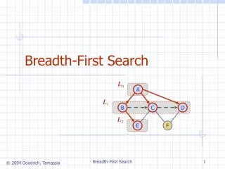
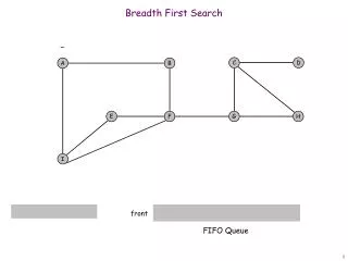
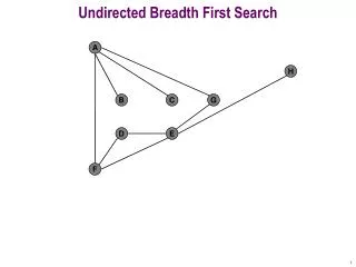
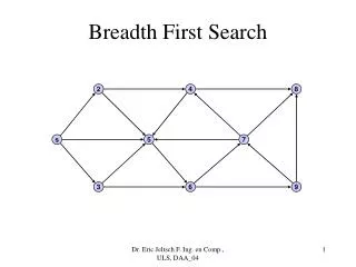
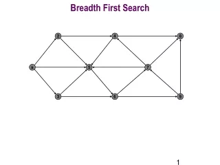
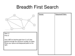
Breadth-first Search (BFS) This method of traversing the graph nodes requires exploration of all the nodes adjacent to the root node before moving deeper. It visits the nodes level by level. Level synchronized BFS algorithms (used in this experiment) proceed level by level on all processors. The Question: Compare the two different partitioning strategies, 1-D and 2-D, with regard to communication and overall time for BFS. Presented by K. Sheldon March 2011
1-D (vertex) Partitioning It is simpler than 2-D partitioning. The vertices of the adjacency matrix are divided up among the processors. The edges emanating from each vertex are owned by the same processor. The edges emanating from a vertex form its edge list. This is the list of vertex indices in row v of matrix A. Below is an example of a 1-D P-way partition of adjacency matrix A , symmetrically reordered so that vertices owned by the same processor are contiguous.
1-D partitioning (cont.) • The disadvantage here for parallel processing is that the vertices point to vertices in all other processors meaning that the communication requirements between processes are all-to-all. This introduces a great deal of overhead. Presented by K. Sheldon March 2011
2-D (edge) Partitioning It is more complex than 1-D partitioning. Edge partitioning divides up the edges rather than vertices between processors resulting in a partial adjacency matrix owned by each process. The advantage is that any edge in the graph can be followed by moving along the row or column. The vertices are also partitioned so that each vertex is also owned by one processor. A process owns edges incident on its vertexes and some edges that are not. Below is an example of a 2-D (checkerboard) partition of adjacency matrix A , again symmetrically reordered so that vertices owned by the same processor are contiguous. Partitioning is for P=RC processors.
2-D partitioning (cont.) The adjacency matrix is divided into RC block rows and C block columns. The A*i,jis a block owned by processor (i,j) . Each processor owns C blocks. For vertices, processor (i,j) owns vertices in block row (j-1)R+I. For comparison, the 1-D partition is a 2-D case where R=1 or C=1. (P = RC) The edge list for a vertex is a column of the adjacency matrix, A. So each block has partial edge lists. Presented by K. Sheldon March 2011
BFS with 1-D Partitioning Algorithm Highlights: • Start with vsand initialize L (levels or graph distance from vs) • Create set F – frontier vertices owned by the processor • The edge lists of F are merged to form set N, neighboring vertices • Send messages to processes that own vertices in set N to potentially add these vertices to their next F • Receive set N vertices from other processors • Merge to form final N set (remove overlap) • Update L Presented by K. Sheldon March 2011
BFS with 2-D Partitioning Algorithm Highlights: Same as 1-D: • Start with vsand initialize L (levels or graph distance from vs) • Create set F – frontier vertices owned by the process Different: • Send F to processor-column, since a v might have the edge list on another processor. • Receive set F from other processors in the column • Merge to form the complete F set • The edge lists (on this processor) of F are merged to form set N, neighboring vertices Almost the Same as 1-D: • Send messages to processors (in processor row) that own vertices in set N to potentially add these vertices to their next F • Receive set N vertices from other processors (in processor row) • Merge to form final N set (remove duplicates) • Update L Presented by K. Sheldon March 2011
Advantage of 2-D Partitioning The advantage of 2-D over 1-D is: Processor-column and processor-row communications: R and C In 1-D partitioning all P processors are involved. In 2-D partitioning each processor must store edge list information about the other processors in its column. Presented by K. Sheldon March 2011
Experimental Results Message length and timing results based on: • Distributed BFS • Poisson random graphs • Load balanced 1-D and 2-D partitioning • 2-D: R = C= √P • 1-D: R = 1, C = P • 100 pairs randomly generated start and target vertices • Timings are the average of the final 99 trials. • Code run on two different computer systems at LLNL: MCR and BlueGene/L Presented by K. Sheldon March 2011
Conclusions • Project Accomplishments: Demonstrated distributed BFS using Poisson random graphs of large scale and compared performance with 1-D and 2-D partitioning. 2-D partitioning is a useful strategy when the average degree k of the graph is large. • Future Work: Investigate different partitioning methods with other more structured graphs such as those with a large clustering coefficient or scale-free graphs. These are graphs with a few vertices that have a very large degree. Presented by K. Sheldon March 2011
Authors Andy Yoo, Edmond Chow, Keith Henderson, William McLendon, Bruce Hendrickson, and UmitCatelyurek. A scalable distributed parallel breadth-first search algorithm on BlueGene/L. In SC ’05: Proceedings of the 2005 ACM/IEEEconference on Supercomputing, 2005. DOI=10.1109/SC.2005.4.46