Graphs – Breadth First Search

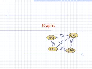
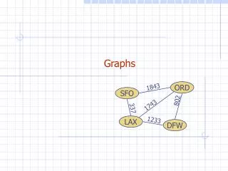
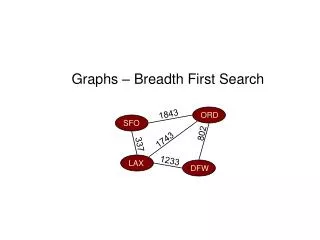
1. Graphs – Breadth First Search 1843 ORD SFO 802 1743 337 1233 LAX DFW

2. Outline BFS Algorithm BFS Application: ShortestPath on an unweighted graph Unweighted Shortest Path: Proof of Correctness

3. Outline BFS Algorithm BFS Application: ShortestPath on an unweighted graph Unweighted Shortest Path: Proof of Correctness

4. Breadth-first search (BFS) is a general technique for traversing a graph A BFS traversal of a graph G Visits all the vertices and edges of G Determines whether G is connected Computes the connected components of G Computes a spanning forest of G BFS on a graph with |V| vertices and |E| edges takes O(|V|+|E|) time BFS can be further extended to solve other graph problems Cycle detection Find and report a path with the minimum number of edges between two given vertices Breadth-First Search

5. BFS Algorithm Pattern

6. BFS is a Level-Order Traversal Notice that in BFS exploration takes place on a wavefront consisting of nodes that are all the same distance from the source s. We can label these successive wavefronts by their distance: L0, L1, …

7. BFS Example undiscovered A A discovered (on Queue) A finished L1 A B C D unexplored edge discovery edge E F cross edge L0 L0 A A L1 L1 B C D B C D E F E F

8. L0 L0 A A L1 L1 B C D B C D L2 E F E F L0 L0 A A L1 L1 B C D B C D L2 L2 E F E F BFS Example (cont.)

9. L0 L0 A A L1 L1 B C D B C D L2 L2 E F E F BFS Example (cont.) L0 A L1 B C D L2 E F

10. Notation Gs: connected component of s Property 1 BFS(G, s) visits all the vertices and edges of Gs Property 2 The discovery edges labeled by BFS(G, s) form a spanning tree Ts of Gs Property 3 For each vertex v in Li The path of Ts from sto vhas i edges Every path from sto vin Gshas at least i edges Properties A B C D E F L0 A L1 B C D L2 E F

11. Setting/getting a vertex/edge label takes O(1) time Each vertex is labeled three times once as BLACK (undiscovered) once as RED (discovered, on queue) once asGRAY (finished) Each edge is considered twice (for an undirected graph) Each vertex is placed on the queue once Thus BFS runs in O(|V|+|E|) time provided the graph is represented by an adjacency list structure Analysis

12. Applications • BFS traversal can be specialized to solve the following problems in O(|V|+|E|) time: • Compute the connected components of G • Compute a spanning forest of G • Find a simple cycle in G, or report that G is a forest • Given two vertices of G, find a path in G between them with the minimum number of edges, or report that no such path exists

13. Outline BFS Algorithm BFS Application: ShortestPath on an unweighted graph Unweighted Shortest Path: Proof of Correctness

14. Application: Shortest Paths on an Unweighted Graph • Goal: To recover the shortest paths from a source node s to all other reachable nodes v in a graph. • The length of each path and the paths themselves are returned. • Notes: • There are an exponential number of possible paths • Analogous to level order traversal for trees • This problem is harder for general graphs than trees because of cycles! ? s

15. Breadth-First Search • Idea: send out search ‘wave’ from s. • Keep track of progress by colouring vertices: • Undiscoveredvertices are colouredblack • Just discovered vertices (on the wavefront) are colouredred. • Previously discovered vertices (behind wavefront) are colouredgrey.

16. BFS Algorithm with Distances and Predecessors

17. First-In First-Out (FIFO) queue stores ‘just discovered’ vertices BFS FoundNot HandledQueue s b a e d g c f j i h m k l

18. BFS FoundNot HandledQueue d=0 s b a s d=0 e d g c f j i h m k l

19. BFS FoundNot HandledQueue d=0 s d=1 b a d=0 a e d=1 d d g g c f b j i h m k l

20. BFS FoundNot HandledQueue d=0 s d=1 b a a d=1 d e d g g b c f j i h m k l

21. BFS FoundNot HandledQueue d=0 s d=1 b a d=1 d e d g g b c f c d=2 j f d=2 i h m k l

22. BFS FoundNot HandledQueue d=0 s d=1 b a d=1 e d g g b c f c d=2 j f d=2 m i e h m k l

23. BFS FoundNot HandledQueue d=0 s d=1 b a d=1 e d g b c f c d=2 j f d=2 m i e h j m k l

24. BFS FoundNot HandledQueue d=0 s d=1 b a d=1 e d g c f c d=2 j f d=2 m i e h j m k l

25. BFS FoundNot HandledQueue d=0 s d=1 b a d=2 c e d f m g e c f j j d=2 i h m k l

26. BFS FoundNot HandledQueue d=0 s d=1 b a d=2 e d f m g e c f j j h d=3 d=2 i i h m d=3 k l

27. BFS FoundNot HandledQueue d=0 s d=1 b a d=2 e d m g e c f j j h d=3 d=2 i i h m d=3 k l

28. BFS FoundNot HandledQueue d=0 s d=1 b a d=2 e d g e c f j j h d=3 d=2 i i h l m d=3 k l

29. BFS FoundNot HandledQueue d=0 s d=1 b a d=2 e d g c f j j h d=3 d=2 i i h l m d=3 k l

30. BFS FoundNot HandledQueue d=0 s d=1 b a d=2 e d g c f j h d=3 d=2 i i h l m d=3 k l

31. BFS FoundNot HandledQueue d=0 s d=1 b a d=3 h i e d l g c f j d=2 i h m d=3 k l

32. BFS FoundNot HandledQueue d=0 s d=1 b a d=3 i e d l g d=4 k c f j d=2 i h m d=3 k d=4 l

33. BFS FoundNot HandledQueue d=0 s d=1 b a d=3 e d l g d=4 k c f j d=2 i h m d=3 k d=4 l

34. BFS FoundNot HandledQueue d=0 s d=1 b a d=3 e d g d=4 k c f j d=2 i h m d=3 k d=4 l

35. BFS FoundNot HandledQueue d=0 s d=1 b a d=4 k e d g c f j d=2 i h m d=3 k d=4 l

36. BFS FoundNot HandledQueue d=0 s d=1 b a d=4 e d=5 d g c f j d=2 i h m d=3 k d=4 l

37. Q is a FIFO queue. Each vertex assigned finite d value at most once. Q contains vertices with d values {i, …, i, i+1, …, i+1} d values assigned are monotonically increasing over time. Breadth-First Search Algorithm: Properties

38. Breadth-First-Search is Greedy • Vertices are handled (and finished): • in order of their discovery (FIFO queue) • Smallest d values first

39. Outline BFS Algorithm BFS Application: ShortestPath on an unweighted graph Unweighted Shortest Path: Proof of Correctness

40. Correctness v & there is an edge from u to v Basic Steps: s d u The shortest path to uhas length d There is a path to v with length d+1.

41. Correctness: Basic Intuition • When we discover v, how do we know there is not a shorter path to v? • Because if there was, we would already have discovered it! s v d u

42. Correctness: More Complete Explanation • Vertices are discovered in order of their distance from the source vertex s. • Suppose that at time t1 we have discovered the set Vd of all vertices that are a distance of d from s. • Each vertex in the set Vd+1 of all vertices a distance of d+1 from s must be adjacent to a vertex in Vd • Thus we can correctly label these vertices by visiting all vertices in the adjacency lists of vertices in Vd. s v d u

43. Correctness: Formal Proof Two-step proof: On exit:

44. s v u

45. v u s

46. x v u s Contradiction!

47. Correctness

48. Progress? • On every iteration one vertex is processed (turns gray).

49. shortest path v u s shortest path shortest path Optimal Substructure Property • The shortest path problem has the optimal substructureproperty: • Every subpath of a shortest path is a shortest path. • The optimal substructure property • is a hallmark of both greedy and dynamic programming algorithms. • allows us to compute both shortest path distance and the shortest paths themselves by storing only one d value and one predecessor value per vertex. How would we prove this?

50. Recovering the Shortest Path For each node v, store predecessor of v inπ(v). s v u π(v) π(v) = u. Predecessor of v is