Graphs
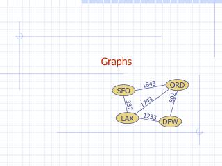
Graphs. 1843. ORD. SFO. 802. 1743. 337. 1233. LAX. DFW. Outline and Reading. Graphs (§6.1) Definitions Applications Terminology Properties ADT Data structures for graphs (§6.2) Edge list structure Adjacency list structure Adjacency matrix structure.

Graphs
E N D
Presentation Transcript
Graphs 1843 ORD SFO 802 1743 337 1233 LAX DFW
Outline and Reading • Graphs (§6.1) • Definitions • Applications • Terminology • Properties • ADT • Data structures for graphs (§6.2) • Edge list structure • Adjacency list structure • Adjacency matrix structure
The Position ADT models the notion of the place within a data structure where a single object is stored It gives a unified view of diverse ways of storing data, such as a cell of an array a node of a linked list Just one method: object element(): returns the element stored at the position Position ADT- Recall from Chpt 2
A graph is a pair (V, E), where V is a set of nodes, called vertices E is a collection of pairs of vertices, called edges Vertices and edges are positions and store elements Edges can be directed or undirected. If all the edges are directed, the graph is called a directed graph or digraph. Graph 849 PVD 1843 ORD 142 SFO 802 LGA 1743 337 1387 HNL 2555 1099 1233 LAX 1120 DFW MIA
Examples of Graphs • Airline route map • Vertices: an airport identified by a three-letter airport code • Edges: a flight route between two airports and specified by the mileage of the route • Flowcharts • These represent the flow of control in a procedure. • Vertices: symbolic flowchart boxes and diamonds • Edges: connecting lines • Binary relations • We say xRy if (x,y) ε SxS, where S is a set. • Vertices: elements in S • Edges: connect x and y iff xRy.
Examples of Graphs • Computer networks • Vertices: computers • Edges: communication links • Electric circuits • Vertices: diodes, transistors, capacitors, switches, ... • Edges: Connecting wires • These examplessuggest the type of questions that can be asked when working with graphs: • What is the cheapest way to fly to NY • What route involves the least flying time? • If one city is closed due to bad weather, does a route to NY exist?
Edge Types • Directed edge • ordered pair of vertices (u,v) • first vertex u is the origin • second vertex v is the destination • e.g., a flight • Undirected edge • unordered pair of vertices (u,v) • e.g., a flight route • Directed graph • all the edges are directed • e.g., flight network • Undirected graph • all the edges are undirected • e.g., route network flight AA 1206 ORD PVD 849 miles ORD PVD
Applications • Electronic circuits • Printed circuit board • Integrated circuit • Transportation networks • Highway network • Flight network • Computer networks • Local area network • Internet • Web • Databases • Entity-relationship diagram
V a b h j U d X Z c e i W g f Y Terminology • End vertices (or endpoints) of an edge • U and V are the endpoints of a • Edges incident on a vertex • a, d, and b are incident on V • Adjacent vertices • U and V are adjacent • Degree of a vertex • X has degree 5 • Parallel edges • h and i are parallel edges • Self-loop • j is a self-loop
Terminology (cont.) • Path • sequence of alternating vertices and edges • begins with a vertex • ends with a vertex • each edge is preceded and followed by its endpoints • Simple path • path such that all its vertices and edges are distinct • Examples • P1=(V,b,X,h,Z) is a simple path • P2=(U,c,W,e,X,g,Y,f,W,d,V) is a path that is not simple V b a P1 d U X Z P2 h c e W g f Y
Terminology (cont.) • Cycle • circular sequence of alternating vertices and edges • each edge is preceded and followed by its endpoints • Simple cycle • cycle such that all its vertices and edges are distinct • Examples • C1=(V,b,X,g,Y,f,W,c,U,a,) is a simple cycle • C2=(U,c,W,e,X,g,Y,f,W,d,V,a,) is a cycle that is not simple V a b d U X Z C2 h e C1 c W g f Y
Notation n number of vertices m number of edges deg(v)degree of vertex v Property 1 Sv deg(v)= 2m Proof: each edge is counted twice Property 2 In an undirected graph with no self-loops and no multiple edges (i.e. a simple graph) m n (n -1)/2 Proof: No 2 edges can have the same endpoints. Thus, each vertex has degree at most (n-1). Thus, by above, 2m≤n(n-1) What is the bound for a directed graph? m≤n(n-1) Proof: No edge can have the same origin and destination. Properties Example • n = 4 • m = 6 • deg(v)= 3
An iterator abstracts the process of scanning through a collection of elements Methods of the ObjectIterator ADT: object object() boolean hasNext() object nextObject() reset() Extends the concept of Position by adding a traversal capability Implement with an array or singly linked list An iterator is typically associated with an another data structure We can augment the Stack, Queue, Vector, List and Sequence ADTs with method: ObjectIterator elements() Two notions of iterator: snapshot: freezes the contents of the data structure at a given time dynamic: follows changes to the data structure Iterator ADT- Recall from Chpt 2
v=vertex & e=edge are positions store elements (o) Update methods insertVertex(o) insertEdge(v, w, o) insertDirectedEdge(v, w, o) removeVertex(v) removeEdge(e) makeUndirected(e) reverseDirection(e) setDirectionFrom(e,v) setDirectionTo(e,v) Generic methods numVertices() numEdges() vertices() edges() See pages 294 and 295 for definitions, although most are obvious. Color key: Returns an iterator Boolean Main Methods of the Graph ADT
Accessor methods aVertex() - returns any vertex as a graph may not have a special vertex incidentEdges(v) adjacentEdges(v) endVertices(e) opposite(v, e) areAdjacent(v, w) degree(v) See pages 294 and 295 for definitions, although most are obvious. Color key: Returns an iterator Boolean Needed for graphs with directed edges directedEdges() undirectedEdges() origin(e) destination(e) isDirected(e) Relating methods inDegree(v) outDegree(v) inIncidentEdges(v) outIncidentEdges(v) inAdjacentVertices(v) outAdjacentVertices(v) Main Methods of the Graph ADT
Why are there so many methods for graphs? • Graphs are very rich and versatile structures. • Therefore, the number of methods is unavoidable when describing the needed methods. • Realize that graphs support two kinds of positions - vertices and edges. • Moreover, edges can be directed or undirected. • Consequently, we need different methods for accessing and updating all these different positions as well as handling relationships between the different positions.
Data Structures for Graphs • Most commonly used • Edge list structure • Adjacency list structure • Adjacency matrix structure • Each has its own strengths and weaknesses in terms of what methods are easier to use and the cost of storage space. • The edge list and the adjacency list actually store representations of the edges. • The adjacency matrix format only uses a placeholder for every pair of vertices. • This implies, as we will see, that the list structures use O(n+m) space and matrix format uses O(n2) where n is number of vertices and m is number of edges.
The Sequence ADT is the union of the Vector and List ADTs Elements accessed by Rank, or Position Generic methods: size(), isEmpty() Vector-based methods: elemAtRank(r), replaceAtRank(r, o), insertAtRank(r, o), removeAtRank(r) List-based methods: first(), last(), before(p), after(p), replaceElement(p, o), swapElements(p, q), insertBefore(p, o), insertAfter(p, o), insertFirst(o), insertLast(o), remove(p) Bridge methods: atRank(r), rankOf(p) Sequence ADT Recall from Chpt 2
Applications of Sequences • The Sequence ADT is a basic, general-purpose, data structure for storing an ordered collection of elements • Direct applications: • Generic replacement for stack, queue, vector, or list • small database (e.g., address book) • Indirect applications: • Building block of more complex data structures
Edge List Structure u • Vertex sequence • sequence of vertex objects • Vertex object • element • reference to position in vertex sequence • Edge object • element • origin vertex object • destination vertex object • reference to position in edge sequence • Edge sequence • sequence of edge objects • Note: Works for both directed and undirected graphs. a c b d v w z z w u v a b c d
Edge List Structure - Notes • This is the simplest and most used data structure for a graph. • The vertex and edge sequence could be a list, vector, or dictionary. • If we use a vector representation, we could think of the vertices as being numbered. • Vertex and edge objects may contain additional information, especially for graphs with some directed edges i,e, an edge vertex could have a Boolean variable indicating whether or not it was directed. • Main feature: Provides direct access from edges to the vertices to which they are incident. • But, accessing the edges that are incident on a vertex requires that all edges be examined. • Obviously, performance of the various methods is very dependent upon which representation is chosen.
Adjacency List Structure a v b • Vertex sequence • sequence of vertex objects • Vertex object • element • reference to position in vertex sequence • reference to incident object • Incidence sequence for each vertex • sequence of references to edge objects of incident edges • Augmented edge objects • references to associated positions in incidence sequences of end vertices u w w u v b a
Adjacency List Structure - Notes • Typically the incident sequence is implemented as a list, but could use a dictionary or a priority queue if their characteristics are useful. • Structure provides direct access from both the edges to the vertices and from the vertices to their incident edges. • Structure matches the performance of the edge list representation, but has improved running time when the above characteristic can be exploited - i.e. given a vertex, return an iterator of incident edges.
Adjacency Matrix Structure a v b • Vertex list structure • Augmented vertex objects • Integer key (index) associated with vertex • 2D adjacency array • Reference to edge object for adjacent vertices • Null for non nonadjacent vertices • The “old fashioned” version just has 0 for no edge and 1 for edge • Edge objects • Edge list structure u w 2 w 0 u 1 v b a
Notes for Adjacency Matrix • Historically, the adjacency matrix was the first represented as a Boolean matrix with A[i,j] = 1 if an edge existed between vertex i and j and 0 otherwise. • The representation shown here updates this to a more object-oriented environment where you use an interface to access the structure. • In all of these structures, additional data may be stored in vertex or edge objects. For example, if edges are being used in a problem about distances between to cities, those distances could be stored in the edge objects.
A B D E C Depth-First Search
Outline and Reading • Definitions (§6.1) • Subgraph • Connectivity • Spanning trees and forests • Depth-first search (§6.3.1) • Algorithm • Example • Properties • Analysis • Applications of DFS (§6.5) • Path finding • Cycle finding
Subgraphs • A subgraph S of a graph G is a graph such that • The vertices of S are a subset of the vertices of G • The edges of S are a subset of the edges of G • A spanning subgraph of G is a subgraph that contains all the vertices of G Subgraph Spanning subgraph
A graph is connected if there is a path between every pair of vertices A connected component of a graph G is a maximal connected subgraph of G Connectivity Connected graph Non connected graph with two connected components
Trees and Forests • A (free) tree is an undirected graph T such that • T is connected • T has no cycles This definition of tree is different from the one of a rooted tree • A forest is an undirected graph without cycles • The connected components of a forest are trees Tree Forest
Spanning Trees and Forests • A spanning tree of a connected graph is a spanning subgraph that is a tree • A spanning tree is not unique unless the graph is a tree • Spanning trees have applications to the design of communication networks • A spanning forest of a graph is a spanning subgraph that is a forest Graph Spanning tree
Traversing a Graph • A traversal of a graph is a systematic procedure for exploring a graph by examining all of its vertices and edges. • Example: • Web spider or crawler is the data collecting part of a search engine that visits all the hypertext documents on the web. (The documents are vertices and the hyperlinks are the edges).
Depth-first search (DFS) is a general technique for traversing a graph A DFS traversal of a graph G does the following: Visits all the vertices and edges of G Determines whether G is connected Computes the connected components of G Computes a spanning forest of G DFS on a graph with n vertices and m edges takes O(n + m ) time DFS can be further extended to solve other graph problems Find and report a path between two given vertices Find a cycle in the graph Depth-first search is to graphs what Euler tour is to binary trees Depth-First Search
Depth-First Search • DFS utilizes backtracking as you would if you were wandering through a maze. • Start at a vertex in G with string; attached the string at the vertex; mark the vertex as "visited". • Explore G by moving out along the incident edges according to some predetermined scheme for ordering and unroll the string. • If you can move to a new vertex, mark it as "visited". • If you hit a "visited" node, backtrack to the last vertex rolling up the string as you go and see if we can move out from there. • The process terminates when the backtracking returns to the place where the string was attached - i.e. the start vertex.
Depth-First Search • It's useful to distinguish edges by their use: • Discovery (or tree) edges - those that are followed to discover new vertices. • Back edges - those that lead to already visited vertices. • For back edges, you need to backtrack to the last visited node and decide if you can move out from it without hitting a visited node. • The discovery edges form a spanning tree of the connected components of the starting vertex - called a DFS tree. • The back edges are also useful - assuming the DFS tree is rooted at the starting vertex, each back edge leads back from a vertex in the tree to one of its ancestors in the tree.
A B D E C A A B D E B D E C C Example unexplored vertex A visited vertex A unexplored edge discovery edge back edge
A A A B D E B D E B D E C C C A B D E C Example (cont.)
DFS and Maze Traversal • The DFS algorithm is similar to a classic strategy for exploring a maze • We mark each intersection, corner and dead end (vertex) visited • We mark each corridor (edge ) traversed • We keep track of the path back to the entrance (start vertex) by means of a rope (recursion stack)
Often Posed as Programming Contest Problem • Given a maze represented as follows: 1=wall , -1=exit. Start at the bottom. To walk systematically, we'll try to go N, W, E, S
Often Posed as Programming Contest Problem • Given a maze represented as follows: 1=wall , -1=exit. Start at the bottom. To walk systematically, we'll try to go N, W, E, S
Often Posed as Programming Contest Problem • Given a maze represented as follows: 1=wall , -1=exit. Start at the bottom. To walk systematically, we'll try to go N, W, E, S
Often Posed as Programming Contest Problem • Given a maze represented as follows: 1=wall , -1=exit. Start at the bottom. To walk systematically, we'll try to go N, W, E, S
Often Posed as Programming Contest Problem • Given a maze represented as follows: 1=wall , -1=exit. Start at the bottom. To walk systematically, we'll try to go N, W, E, S
Often Posed as Programming Contest Problem • Given a maze represented as follows: 1=wall , -1=exit. Start at the bottom. To walk systematically, we'll try to go N, W, E, S
Often Posed as Programming Contest Problem • Given a maze represented as follows: 1=wall , -1=exit. Start at the bottom. To walk systematically, we'll try to go N, W, E, S
Often Posed as Programming Contest Problem • Given a maze represented as follows: 1=wall , -1=exit. Start at the bottom. To walk systematically, we'll try to go N, W, E, S
Often Posed as Programming Contest Problem • Given a maze represented as follows: 1=wall , -1=exit. Start at the bottom. To walk systematically, we'll try to go N, W, E, S
Often Posed as Programming Contest Problem • Given a maze represented as follows: 1=wall , -1=exit. Start at the bottom. To walk systematically, we'll try to go N, W, E, S
Often Posed as Programming Contest Problem • Given a maze represented as follows: 1=wall , -1=exit. Start at the bottom. To walk systematically, we'll try to go N, W, E, S The exact path taken depends on this ordering.