Download
1 / 84
840 likes | 1.03k Vues
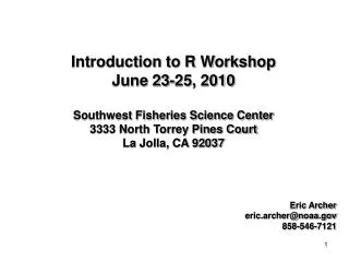
Introduction to R Workshop June 23-25, 2010 Southwest Fisheries Science Center 3333 North Torrey Pines Court La Jolla, CA 92037. Eric Archer eric.archer@noaa.gov 858-546-7121. Introduction to R. 1) How R thinks Environment Data Structures Data Input/Output. 2) Becoming a codeR

E N D
Introduction to R Workshop June 23-25, 2010 Southwest Fisheries Science Center 3333 North Torrey Pines CourtLa Jolla, CA 92037 Eric Archer eric.archer@noaa.gov 858-546-7121
Introduction to R • 1) How R thinks • Environment • Data Structures • Data Input/Output • 2) Becoming a codeR • Data Selection and Manipulation • Data Summary • Functions • 3) Visualization and analysis • Data Processing (‘apply’ family) • Plotting & Graphics • Statistical Distributions • Statistical Tests • Model Fitting • Packages, Path, Options
S, S-Plus, R S-Plus 1988: Statistical Sciences 1993: MathSoft 2001: Insightful 2008: TIBCO S Chambers, Becker, Wilks 1984: Bell Labs R Ihaka & Gentleman 1996 (The R Project) • Why R? • Free • Open source • Many packages • Large support base • Multi-platform • Vectorization “Programming ought to be regarded as an integral part of effective and responsible data analysis” - Venables and Ripley. 1999. S Programming
Workspace • Entering commands • commands and assignments executed or evaluated immediately • separated by new line (Enter/Return) or semicolon • recall commands with ↑ or ↓ • case sensitive • everything is some sort of function that does something • Getting help • > help(mean) > ?median > help(“[“) • > example(mean) • > help.search(“regression”) • > RSiteSearch(“genetics”) • > http://www.r-project.org/
Workspace ls() list objects in workspace rm(…) remove objects from workspace rm(list = ls()) remove all objects from workspace save.image() saves workspace load(".rdata") loads saved workspace history() view command history loadhistory() load command history savehistory() save command history # comments
Assignment and data creation <- assign c(…) combine arguments into a vector seq(x) generate sequence from 1 to x seq(from,to,by) generate sequence with increment by from:to generate sequence from .. to rep(x,times) replicate x letters,LETTERS vector of 26 lower and upper case letters > x <- 1 > y <- "A" > my.vec <- c(1, 5, 6, 10) > my.nums <- 12:24 > x [1] 1 > y [1] "A" > my.vec [1] 1 5 6 10 > my.nums [1] 12 13 14 15 16 17 18 19 20 21 22 23 24
Data Structures Object modes (atomic structures) integer whole numbers (15, 23, 8, 42, 4, 16) numeric real numbers (double precision: 3.14, 0.0002, 6.022E23) character text string (“Hello World”, “ROFLMAO”, “A”) logical TRUE/FALSE or T/F Object classes vector object with atomic mode factor vector object with discrete groups (ordered/unordered) array multiple dimensions matrix 2-dimensional array list vector of components data.frame "matrix –like" list of variables of same # of rows Special Values NULL object of zero length, test with is.null(x) NA Not Available / missing value, test with is.na(x) NaN Not a number, test with is.nan(x) (e.g. 0/0, log(-1)) Inf, -Inf Positive/negative infinity, test with is.infinite(x) (e.g. 1/0)
Vectors Creation and info vector(mode,length) create vector length(x) number of elements names(x) get or set names Indexing (number, character (name), or logical) x[n] nth element x[-n] all but the nth element x[a:b] elements a to b x[-(a:b)] all but elements a to b x[c(…)] specific elements x[“name”]“name” element x[x > a] all elements greater than a x[x %in% c(…)] all elements in the set
Vectors Create a vector > x <- 1:10 Give the elements some names > names(x) <- c("first","second","third","fourth","fifth") Select elements based on another vector > i <- c(1,5) > x[i] first fifth 1 5 > x[-c(i,8)] second third fourth <NA> <NA> <NA> <NA> 2 3 4 6 7 9 10
logical testing == equals >, < greater, less than >=, <= greater,less than or equal to ! not &, && and (single is element-by-element, double is first element) |, || or Vectors Select elements based on a condition > x <- 1:10 > x[x < 5] [1] 1 2 3 4 > x < 5 [1] TRUE TRUE TRUE TRUE FALSE FALSE FALSE FALSE FALSE FALSE > x[x < 5] [1] 1 2 3 4 & vs && > x < 5 & x > 2 [1] FALSE FALSE TRUE TRUE FALSE FALSE FALSE FALSE FALSE FALSE > x < 5 && x > 2 [1] FALSE
Vectorization Operator recycles smaller object enough times to cover larger object > x <- 4 > y <- c(5, 6, 7, 8, 9, 10) > z <- x + y > z [1] 9 10 11 12 13 14 > x <- c(3,5) > z <- x+y > z [1] 8 11 10 13 12 15 > i <- 1:10 > j <- c(T,T,F) > i[j] [1] 1 2 4 5 7 8 10
Object Information summary(x) generic summary of object str(x) display object structure mode(x) get or set storage mode class(x) name of object class is.<class>(x) test type of object (is.numeric, is.logical, etc.) attr(x, which) get or set the attribute of an object attributes(x) get or set all attributes of an object
Object Information > y <- 1:10 > str(y) int [1:10] 1 2 3 4 5 6 7 8 9 10 > mode(y) [1] "numeric“ > class(y) [1] "integer“ > is.character(y) [1] FALSE > is.integer(y) [1] TRUE > is.double(y) [1] FALSE > is.numeric(y) [1] TRUE
Object Information > x <- 1:4 > names(x) <- c("first","second","third","four") > x first second third four 1 2 3 4 > str(x) Named int [1:4] 1 2 3 4 - attr(*, "names")= chr [1:4] "first" "second" "third" "four" > attributes(x) $names [1] "first" "second" "third" "four" > attr(x, "notes") <- "This is a really important vector." > attributes(x) $names [1] "first" "second" "third" "four" $notes [1] "This is a really important vector." > attr(x, "date") <- 20090624 > attributes(x) $names [1] "first" "second" "third" "four" $notes [1] "This is a really important vector." $date [1] 20090624 > x first second third four 1 2 3 4 attr(,"notes") [1] "This is a really important vector." attr(,"date") [1] 20090624
coercion as.<class>(x) coerces object x to <class> if possible > x <- 1:10 > x.char <- as.character(x) > as.numeric(x.char) [1] 1 2 3 4 5 6 7 8 9 10 > y <- letters[1:10] > as.numeric(y) [1] NA NA NA NA NA NA NA NA NA NA Warning message: NAs introduced by coercion > z <- "1char" > as.numeric(z) [1] NA Warning message: NAs introduced by coercion > logic.chars <- c("TRUE", "FALSE", "T", "F", "t", "f", "0", "1") > as.logical(logic.chars) [1] TRUE FALSE TRUE FALSE NA NA NA NA > logic.nums <- c(-2, -1, 0, 1.5, 2, 100) > as.logical(logic.nums) [1] TRUE TRUE FALSE TRUE TRUE TRUE
Factors • Discrete ordered or unordered data • Internally represented numerically • factor(x, levels, labels, exclude, ordered) • levels(x) • labels(x) • is.factor(x),is.ordered(x)
Factors > x <- c("b", "a", "a", "c", "B", "d", "a", "d") > x.fac <- factor(x) > x.fac [1] b a a c B d a d Levels: a b B c d > str(x.fac) Factor w/ 5 levels "a","b","B","c",..: 2 1 1 4 3 5 1 5 > levels(x.fac) [1] "a" "b" "B" "c" "d“ > labels(x.fac) [1] "1" "2" "3" "4" "5" "6" "7" "8“ > as.numeric(x.fac) [1] 2 1 1 4 3 5 1 5 > as.character(x.fac) [1] "b" "a" "a" "c" "B" "d" "a" "d"
Factors > x.fac.lvl <- factor(x, levels = c("a", "c")) > x.fac.lvl [1] <NA> a a c <NA> <NA> a <NA> Levels: a c > x.fac.exc <- factor(x, exclude = c("a", "c")) > x.fac.exc [1] b <NA> <NA> <NA> B d <NA> d Levels: b B d > x.fac.lbl <- factor(x, labels = c("L1", "L2", "L3", "L4", "L5")) > x.fac.lbl [1] L2 L1 L1 L4 L3 L5 L1 L5 Levels: L1 L2 L3 L4 L5 > x.fac[2] < x.fac[1] [1] NA Warning message: In Ops.factor(x.fac[2], x.fac[1]) : < not meaningful for factors > x.ord <- factor(x, ordered = TRUE) > x.ord [1] b a a c B d a d Levels: a < b < B < c < d > x.ord[2] < x.ord[1] [1] TRUE
Arrays and Matrices array(data, dim, dimnames) create array (row-priority) matrix(data, nrow, ncol, dimnames) create matrix x[row, col] element at row,col x[row,] x[, col] vector of row and col x[“name”, ] vector of row “name” etc. dim(x) retrieve or set dimensions nrow(x) number of rows ncol(x) number of columns dimnames(x) retrieve or set dimension names rownames(x) retrieve or set row names colnames(x) retrieve or set column names cbind(…) create array from columns rbind(…) create array from rows t(x) transpose (matrices)
Arrays and Matrices Create an array > x <- array(1:10, dim = c(4, 6)) > x [,1] [,2] [,3] [,4] [,5] [,6] [1,] 1 5 9 3 7 1 [2,] 2 6 10 4 8 2 [3,] 3 7 1 5 9 3 [4,] 4 8 2 6 10 4 > str(x) int [1:4, 1:6] 1 2 3 4 5 6 7 8 9 10 ... > attributes(x) $dim [1] 4 6 > dim(x) [1] 4 6 > dimnames(x) NULL
Arrays and Matrices Set column or row names > colnames(x) <- c("col1", "col2", "col3", "col4", "5", "6") > x col1 col2 col3 col4 5 6 [1,] 1 5 9 3 7 1 [2,] 2 6 10 4 8 2 [3,] 3 7 1 5 9 3 [4,] 4 8 2 6 10 4 > colnames(x) <- c("column1", "column2") Error in dimnames(x) <- dn : length of 'dimnames' [2] not equal to array extent > colnames(x)[1] <- "column1" > x column1 col2 col3 col4 5 6 [1,] 1 5 9 3 7 1 [2,] 2 6 10 4 8 2 [3,] 3 7 1 5 9 3 [4,] 4 8 2 6 10 4
Set row and columns names using dimnames > dimnames(x) <- list(c("first", "second", "third", "4"), NULL) > x [,1] [,2] [,3] [,4] [,5] [,6] first 1 5 9 3 7 1 second 2 6 10 4 8 2 third 3 7 1 5 9 3 4 4 8 2 6 10 4 Arrays and Matrices Setting dimension names > dimnames(x) <- list(my.rows = c("first", "second", "third", "4"), my.cols = NULL) > x my.cols my.rows [,1] [,2] [,3] [,4] [,5] [,6] first 1 5 9 3 7 1 second 2 6 10 4 8 2 third 3 7 1 5 9 3 4 4 8 2 6 10 4
Change dimensionality of array > dim(x) <- c(6, 4) > x [,1] [,2] [,3] [,4] [1,] 1 7 3 9 [2,] 2 8 4 10 [3,] 3 9 5 1 [4,] 4 10 6 2 [5,] 5 1 7 3 [6,] 6 2 8 4 > dim(x) <- c(3, 4, 2) > x , , 1 [,1] [,2] [,3] [,4] [1,] 1 4 7 10 [2,] 2 5 8 1 [3,] 3 6 9 2 , , 2 [,1] [,2] [,3] [,4] [1,] 3 6 9 2 [2,] 4 7 10 3 [3,] 5 8 1 4 Arrays
Arrays and Matrices Bind several vectors into an array > i1 <- seq(from = 1, to = 20, length = 10) > i2 <- seq(from = 3.4, to = 25, length = 10) > i3 <- seq(from = 15, to = 25, length = 10) > i <- cbind(i1, i2, i3) > i i1 i2 i3 [1,] 1.000000 3.4 15.00000 [2,] 3.111111 5.8 16.11111 [3,] 5.222222 8.2 17.22222 [4,] 7.333333 10.6 18.33333 [5,] 9.444444 13.0 19.44444 [6,] 11.555556 15.4 20.55556 [7,] 13.666667 17.8 21.66667 [8,] 15.777778 20.2 22.77778 [9,] 17.888889 22.6 23.88889 [10,] 20.000000 25.0 25.00000
Arrays and Matrices > j <- rbind(i1, i2, i3) > j [,1] [,2] [,3] [,4] [,5] [,6] [,7] [,8] [,9] i1 1.0 3.111111 5.222222 7.333333 9.444444 11.55556 13.66667 15.77778 17.88889 i2 3.4 5.800000 8.200000 10.600000 13.000000 15.40000 17.80000 20.20000 22.60000 i3 15.0 16.111111 17.222222 18.333333 19.444444 20.55556 21.66667 22.77778 23.88889 [,10] i1 20 i2 25 i3 25 > i <- cbind(col1 = i1, col2 = i2, col3 = i3)
Lists • Special vector • Collection of elements of different modes • Often used as return type of functions • list(…), vector(“list”, length)create list • x[i] list of element i • x[[i]] element i • x[“name”]list of element name • x[[“name”]] or x$name element name • unlist transform list to a vector
Lists > x <- list(1:10, c("a", "b"), c(TRUE, TRUE, FALSE, TRUE), 5) > x [[1]] [1] 1 2 3 4 5 6 7 8 9 10 [[2]] [1] "a" "b" [[3]] [1] TRUE TRUE FALSE TRUE [[4]] [1] 5 > is.list(x) [1] TRUE > is.vector(x) [1] TRUE > is.numeric(x) [1] FALSE
Lists What are the elements in a list? > x[1] [[1]] [1] 1 2 3 4 5 6 7 8 9 10 > str(x[1]) List of 1 $ : int [1:10] 1 2 3 4 5 6 7 8 9 10 > mode(x[1]) [1] "list“ > x[[1]] [1] 1 2 3 4 5 6 7 8 9 10 > str(x[[1]]) int [1:10] 1 2 3 4 5 6 7 8 9 10 > mode(x[[1]]) [1] "numeric“
Lists > y <- list(numbers = c(5, 10:25), initials = c(“rnm", "fds")) > y $numbers [1] 5 10 11 12 13 14 15 16 17 18 19 20 21 22 23 24 25 $initials [1] “rnm" "fds" > y$initials [1] “rnm" "fds“ > y["numbers"] $numbers [1] 5 10 11 12 13 14 15 16 17 18 19 20 21 22 23 24 25 > y$new.element <- "This is new" > y $numbers [1] 5 10 11 12 13 14 15 16 17 18 19 20 21 22 23 24 25 $initials [1] “rnm" "fds" $new.element [1] "This is new"
Data Frames • Like matrices, but columns of different modes • Organized list where components are columns of equal length rows • x[[“name”]] or x$name column name • x[row, column], etc. • > age <- c(1:5) • > color <- c("neonate", "two-tone", "speckled", "mottled", "adult") • > juvenile <- c(TRUE, TRUE, FALSE, FALSE, FALSE) • > spotted <- data.frame(age, color, juvenile) • > spotted • age color juvenile • 1 1 neonate TRUE • 2 2 two-tone TRUE • 3 3 speckled FALSE • 4 4 mottled FALSE • 5 adult FALSE
Data Frames > is.matrix(spotted) [1] FALSE > is.array(spotted) [1] FALSE > is.list(spotted) [1] TRUE > is.data.frame(spotted) [1] TRUE > spotted$age [1] 1 2 3 4 5 > spotted$age[2] [1] 2 > spotted$color[2] [1] two-tone Levels: adult mottled neonate speckled two-tone > spotted[spotted$age < 3, ] age color juvenile 1 1 neonate TRUE 2 2 two-tone TRUE
Data Frames Forcing character columns > str(spotted) 'data.frame': 5 obs. of 3 variables: $ age : int 1 2 3 4 5 $ color : Factor w/ 5 levels "adult","mottled",..: 3 5 4 2 1 $ juvenile: logi TRUE TRUE FALSE FALSE FALSE > spotted2 <- data.frame(age.class = age, + color.pattern = color, juvenile.stat = juvenile, + stringsAsFactors = FALSE) > spotted2 age.class color.pattern juvenile.stat 1 1 neonate TRUE 2 2 two-tone TRUE 3 3 speckled FALSE 4 4 mottled FALSE 5 5 adult FALSE > str(spotted2) 'data.frame': 5 obs. of 3 variables: $ age.class : int 1 2 3 4 5 $ color.pattern: chr "neonate" "two-tone" "speckled" "mottled" ... $ juvenile.stat: logi TRUE TRUE FALSE FALSE FALSE
Data Frames Deleting columns > spotted$age <- NULL > spotted color juvenile 1 neonate TRUE 2 two-tone TRUE 3 speckled FALSE 4 mottled FALSE 5 adult FALSE Creating new columns > spotted$freq <- c(0.3, 0.2, 0.2, 0.15, 0.15) > spotted$have.data <- TRUE > spotted color juvenile freq have.data 1 neonate TRUE 0.30 TRUE 2 two-tone TRUE 0.20 TRUE 3 speckled FALSE 0.20 TRUE 4 mottled FALSE 0.15 TRUE 5 adult FALSE 0.15 TRUE
Data Frames subset(x, subset, select) > subset(spotted, age >=3) age color juvenile 3 3 speckled FALSE 4 4 mottled FALSE 5 5 adult FALSE > subset(spotted, juvenile == FALSE & age <= 4) age color juvenile 3 3 speckled FALSE 4 4 mottled FALSE > subset(spotted, age <=2, select = c("color", "juvenile")) color juvenile 1 neonate TRUE 2 two-tone TRUE
Data Input/Output Directory management dir() list files in directory setwd(path) set working directory getwd() get working directory ?files File and Directory Manipulation Standard ASCII Format read.table creates a data frame from text file read.csv read comma-delimited file read.delim read tab-delimited file read.fwf read fixed width format write.table write data to text file write.csv write comma-delimited file R Binary Format save writes binary R objects save.image writes current environment in binary R load reload files written with save R Text Format dump creates text representation of R objects source accept input from text file (scripts)
Data Input/Output Reading ASCII > sets <- read.csv("Sets_All.csv", header = TRUE) > sets$Ordered.Year <- ordered(sets$Year) > sets$SpotCd.Fac <- factor(sets$SpotCd, exclude = NULL) > spotted.sets <- sets[sets$Sp1Cd == 2, ] > write.table(spotted.sets, file = "spotted.txt", + row.names = FALSE) Reading R binary > save(spotted.sets, file = "spotted.RData") > rm(list = ls()) > load("spotted.RData") Reading R commands > positions <- spotted.sets[, c("Latitude", "Longitude")] > dump("positions", file = "set_positions.R") > rm(list = ls()) > source("set_positions.R")
Writing Scripts • Text files containing commands and comments written as if executed on command line (usually end with .r) • From R GUI : File|New script • Any text editor (Notepad, Tinn-R, VEDIT, etc.) • Commands executed with: • source("filename.r") • Copy/paste • From R Editor : Edit|Run...
Exercise 1A : Assemble data frame • Assemble a data frame from “Homework 1” files with only these columns (make these names and in this order): boat (character), skipper (character), lat, lon, year, month, day, mammals, turtles, fish • Add a column classifying each trip by season: Winter: Dec – Feb, Spring: Mar – May, Summer: Jun – Aug, Fall: Sep – Nov • Add three columns classifying bycatch size for each of: • fish : < 15 (small), 15 – 200 (medium), > 200 (large) • turtles : < 4 (small), >= 4 (large) • mammals: < 2 (small), >= 2 (large) • 4. Add column indicating that boat needs to be inspected if any bycatch class is “large” • 5. Write your new data frame to a .csv file Exercise 1B : Make a list • Read .csv file from 1A into clean R environment • Create a list with one element for the entire data set and one element per bycatch type (4 elements total). Each bycatch element should contain a named vector of the number of trips with small, medium, and large bycatches • How many trips needed to be inspected? • How many trips had no bycatch at all? • Save list and results from 3 & 4 in an R workspace End Day 1
Data Selection and Manipulation sample(x, size, replace, prob) take a random sample from x cut(x, breaks, labels) divide vector into intervals %in% return logical vector of matches which(x) return index of TRUE results all(…), any(…) return TRUE if all or any arguments are TRUE unique(x) return unique observations in vector duplicated(x) return duplicated observations sort sort vector or factor order sort based on multiple arguments merge() merge two data frames by common cols or rows ceiling, floor, trunc, round, signif rounding functions
sample > x <- 1:5 Sample x (jumble or permute) > sample(x) [1] 2 1 4 5 3 Sample from x > sample(x, 3) [1] 2 4 3 Sample with replacement > sample(x, 10, replace = TRUE) [1] 2 3 5 3 3 4 2 1 4 4 Sample with modified probabilities > cars <- c("Ford", "GM", "Toyota", "VW", "Subaru", "Honda") > male.wts <- c(6, 5, 3, 1, 3, 3) > female.wts <- c(3, 3, 4, 8, 3, 6) > > male.survey <- sample(cars, 100, replace = TRUE, prob = male.wts) > female.survey <- sample(cars, 100, replace = TRUE, prob = female.wts)
cut cut(x, breaks, labels = NULL, include.lowest = FALSE, right = TRUE, dig.lab = 3, ordered_result = FALSE, ...) > y <- c(4, 5, 6, 10, 11, 30, 49, 50, 51) Bins : 5 > y <= 10, 10 > y <= 30, 30 > y <= 50 > y.cut <- cut(y, breaks = c(5, 10, 30, 50)) > y.cut [1] <NA> <NA> (5,10] (5,10] (10,30] (10,30] (30,50] (30,50] <NA> Levels: (5,10] (10,30] (30,50] > str(y.cut) Factor w/ 3 levels "(5,10]","(10,30]",..: NA NA 1 1 2 2 3 3 NA Bins : 5 >= y <= 10, 10 > y <= 30, 30 > y <= 50 > cut(y, breaks = c(5, 10, 30, 50), include.lowest = TRUE) [1] <NA> [5,10] [5,10] [5,10] (10,30] (10,30] (30,50] (30,50] <NA> Levels: [5,10] (10,30] (30,50] Bins : 5 >= y < 10, 10 >= y < 30, 30 >= y < 50 > cut(y, breaks = c(5, 10, 30, 50), right = FALSE) [1] <NA> [5,10) [5,10) [10,30) [10,30) [30,50) [30,50) <NA> <NA> Levels: [5,10) [10,30) [30,50) Bins : 5 >= y < 10, 10 >= y < 30, 30 >= y <= 50 > cut(y, breaks = c(5, 10, 30, 50), include.lowest = TRUE, right = FALSE) [1] <NA> [5,10) [5,10) [10,30) [10,30) [30,50] [30,50] [30,50] <NA> Levels: [5,10) [10,30) [30,50]
%in%, which > x <- sample(1:10, 20, replace = TRUE) > x [1] 4 10 2 3 4 3 6 4 7 3 9 1 3 4 7 1 3 2 8 [20] 5 > x %in% c(3, 10, 2, 1) [1] FALSE TRUE TRUE TRUE FALSE TRUE FALSE FALSE FALSE [10] TRUE FALSE TRUE TRUE FALSE FALSE TRUE TRUE TRUE [19] FALSE FALSE > x[x %in% c(3, 10, 2, 1)] [1] 10 2 3 3 3 1 3 1 3 2 > which(x %in% c(3, 10, 2, 1)) [1] 2 3 4 6 10 12 13 16 17 18 > which(x < 5) [1] 1 3 4 5 6 8 10 12 13 14 16 17 18 > x[which(x > 6)] [1] 10 7 9 7 8
any, all > x <- sample(1:10, 20, replace = TRUE) > x [1] 2 7 8 1 1 7 5 8 6 7 3 7 2 1 5 10 3 9 1 2 > any(x == 6) [1] TRUE > all(x < 5) [1] FALSE
unique, duplicated > x <- sample(1:10, 20, replace = TRUE) > x [1] 6 5 1 8 9 6 2 3 8 9 8 10 10 2 9 3 4 3 4 [20] 10 > unique(x) [1] 6 5 1 8 9 2 3 10 4 > duplicated(x) [1] FALSE FALSE FALSE FALSE FALSE TRUE FALSE FALSE TRUE [10] TRUE TRUE FALSE TRUE TRUE TRUE TRUE FALSE TRUE [19] TRUE TRUE
sort, order > x <- sample(1:10, 20, replace = TRUE) > x [1] 3 6 7 1 5 3 10 3 7 2 3 9 1 8 4 3 8 2 [19] 4 1 > sort(x) [1] 1 1 1 2 2 3 3 3 3 3 4 4 5 6 7 7 8 8 [19] 9 10 > sort(x, decreasing = TRUE) [1] 10 9 8 8 7 7 6 5 4 4 3 3 3 3 3 2 2 1 [19] 1 1 > order(x) [1] 4 13 20 10 18 1 6 8 11 16 15 19 5 2 3 9 14 17 [19] 12 7 > trips <- read.csv(“homework 1a df.csv") > month.sort <- trips[order(trips$month), ] > month.days.sort <- trips[order(trips$month, trips$day), ]
merge merge(x, y, by = intersect(names(x), names(y)), by.x = by, by.y = by, all = FALSE, all.x = all, all.y = all, sort = TRUE, suffixes = c(".x",".y"), ...) > rm(list = ls()) > load("merge data.rdata") > str(cranial) 'data.frame': 20 obs. of 2 variables: $ id : Factor w/ 20 levels "Specimen-1","Specimen-12",..: 14 11 13 7 20 18 3 10 5 17 ... $ skull: num 260 266 259 273 262 ... > str(haps) 'data.frame': 20 obs. of 2 variables: $ id : Factor w/ 20 levels "Specimen-1","Specimen-10",..: 16 12 15 18 8 7 3 13 6 9 ... $ haps: Factor w/ 5 levels "A","B","C","D",..: 1 4 4 5 5 3 1 3 3 4 ... > merge(haps, cranial) id haps skull 1 Specimen-1 A 255.4461 2 Specimen-12 A 262.5730 3 Specimen-16 E 256.2258 4 Specimen-22 E 259.2000 ...
merge merge(x, y, by = intersect(names(x), names(y)), by.x = by, by.y = by, all = FALSE, all.x = all, all.y = all, sort = TRUE, suffixes = c(".x",".y"), ...) > str(sex) 'data.frame': 40 obs. of 2 variables: $ specimens: Factor w/ 40 levels "Specimen-1","Specimen-10",..: 1 12 23 34 36 37 38 39 40 2 ... $ sex : Factor w/ 2 levels "F","M": 1 2 1 2 2 2 2 2 2 1 ... > str(trials) 'data.frame': 30 obs. of 2 variables: $ id : Factor w/ 23 levels "Specimen-1","Specimen-18",..: 5 6 1 9 3 7 8 2 10 4 ... $ value: num 30.1 23.1 24.3 22.6 36.7 ... > merge(sex, trials, by.x = "specimens", by.y = "id") specimens sex value 1 Specimen-1 F 24.28745 2 Specimen-11 F 23.90455 3 Specimen-12 M 27.41010 4 Specimen-14 M 36.84547 5 Specimen-15 M 20.08898
String Manipulation nchar(x) number of characters in string substr(x, start, stop) extract or replace substrings strsplit(x, split) split string paste(..., sep, collapse) concatenate vectors format format object for printing grep, sub, gsub pattern matching and replacement
nchar, substr, strsplit > x <- "This is a sentence." > nchar(x) [1] 19 > substr(x, 3, 9) [1] "is is a“ > substr(x, 1, 4) <- "That" > x [1] "That is a sentence.“ > strsplit(x, " ") [[1]] [1] "That" "is" "a" "sentence." > strsplit(x, "a") [[1]] [1] "Th" "t is " " sentence."
paste > sites <- LETTERS[1:6] > paste("Site", sites) [1] "Site A" "Site B" "Site C" "Site D" "Site E" "Site F" > paste("Site", sites, sep = "-") [1] "Site-A" "Site-B" "Site-C" "Site-D" "Site-E" "Site-F" > paste("Site", sites, sep = "_", collapse = ",") [1] "Site_A,Site_B,Site_C,Site_D,Site_E,Site_F"