Arch ( A )
Loop (60%). Arch/Tented Arch (6%). Whorl (34%). Other (Less than 1%) (accidentals). Arch ( A ). Tented Arch ( T ). Loop ( U or R ). Whorl ( W ). The four main classes of fingerprints. Johannes Purkinje 1787-1869. Distribution of classes (Caucasian) .
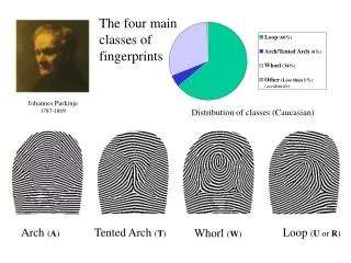

Arch ( A )
E N D
Presentation Transcript
Loop (60%) Arch/Tented Arch (6%) Whorl (34%) Other (Less than 1%) (accidentals) Arch (A) Tented Arch (T) Loop (U or R) Whorl (W) The four main classes of fingerprints Johannes Purkinje 1787-1869 Distribution of classes (Caucasian)
No Normal Class on Thursday!! Instead I will be in my office, and the TAs will be in the TA lab, to answer questions about any section of the material covered since day one. Congratulations to Foula, who passed her qualifying exams with the highest grade!
1) R Thumb 16 1) R Thumb 2) R Index 2) R Index 16 3) R Middle 8 3) R Middle 4) R Ring 8 4) R Ring 8 5) R Little 5) R Little 4 Sir Edward Henry 1850-1931 6) L Thumb 4 6) L Thumb 7) L Index 2 7) L Index 8) L Middle 2 8) L Middle 9) L Ring 1 9) L Ring 1 10) L Little 1 10) L Little 8 + 1 1 + 1 9 2 = The Henry Classification System The sum of the values of the white squares that contain a Whorl (plus one) is the numerator of the primary classification. The sum of the values of the dark squares that contain a Whorl (plus one) is the denominator of the primary classification. U W A U A A U U W U
1) R Thumb 1) R Thumb 2) R Index 2) R Index 3) R Middle 3) R Middle 4) R Ring 4) R Ring 8 5) R Little 5) R Little 6) L Thumb 6) L Thumb 4 7) L Index 7) L Index 2 8) L Middle 8) L Middle 9) L Ring 1 9) L Ring 1 10) L Little 1 10) L Little 10 4 4 + 1 1 + 1 9 + 1 3 + 1 10 4 5 2 = = The Henry Classification System II You cannot “simplify” the classes by canceling above and below the fraction bar. Read as “Ten over Four” not as “ten fourths”
The Henry Classification System III How many different classifications are there? Each finger position has exactly 2 possibilities, either it contains a Whorl or it does not. There are 5 positions in the numerator, so there are 25 possible numerators. The same argument is holds for the denominator. So the number of possible numerators times the number of possible denominators is 25*25 = 210 = 1024 Some of the 1024 “bins” in Scotland Yards Fingerprint Bureau during the 1950s
Static Hashing • A bucket is a unit of storage containing one or more records (a bucket is typically a disk block). • In a hash file organization we obtain the bucket of a record directly from its search-key value using a hashfunction. • Hash function h is a function from the set of all search-key values K to the set of all bucket addresses B. • Hash function is used to locate records for access, insertion as well as deletion. • Records with different search-key values may be mapped to the same bucket; thus entire bucket has to be searched sequentially to locate a record.
Static Hashing With hash based indexing, we assume that we have a function h, which tells us where to place any given record. h ::: Data Page 1 Data Page 2 Data Page 3 Data Page N-1 Data Page N
Static Hashing The hash function usually takes the last k bits of the search key, multiples it by a, and adds b to get some value. The id of the page to access is identified by… page_number = h(value) mod N The values of a and b must be carefully selected, N should be prime. We desired the hash function to uniform and random (explained later).
Static Hashing As with ISAM, insertion can cause overflow. The solution is to create chains of overflow pages. h ::: Data Page 1 Data Page 2 Data Page 3 Data Page N-1 Data Page N Overflow for 3
Note about Notation • Our book, and more generally the world, is inconsistent about notation. The page number that we should place our record in is sometimes given as… • page_number = h(value) mod N • And sometimes as… • page_number = h(value) • There is nothing “deep” going on here, it is just that the “Mod N” has been moved inside the notation in the second case.
Hash Functions • Worst has function maps all search-key values to the same bucket; this makes access time proportional to the number of search-key values in the file. • An ideal hash function is uniform, i.e., each bucket is assigned the same number of search-key values from the set of all possible values. • Ideal hash function is random, so each bucket will have the same number of records assigned to it irrespective of the actual distribution of search-key values in the file. • Typical hash functions perform computation on the internal binary representation of the search-key. • For example, for a string search-key, the binary representations of all the characters in the string could be added and the sum modulo the number of buckets could be returned.
Handling of Bucket Overflows • Bucket overflow can occur because of • Insufficient buckets • Skew in distribution of records. This can occur due to two reasons: • multiple records have same search-key value • chosen hash function produces non-uniform distribution of key values • Although the probability of bucket overflow can be reduced, it cannot be eliminated.
Deficiencies of Static Hashing • In static hashing, function h maps search-key values to a fixed set of B of bucket addresses. • Databases grow with time. If initial number of buckets is too small, performance will degrade due to too much overflows. • If file size at some point in the future is anticipated and number of buckets allocated accordingly, significant amount of space will be wasted initially. • If database shrinks, again space will be wasted. • One option is periodic re-organization of the file with a new hash function, but it is very expensive. • These problems can be avoided by using techniques that allow the number of buckets to be modified dynamically.
Deficiencies of Static Hashing …These problems can be avoided by using techniques that allow the number of buckets to be modified dynamically. • This is called dynamic hashing. • There are several types of dynamic hashing, we will learn about extendible hashing, and linear hashing. • First we must learn about hash indices.
Hash Indices • Hashing can be used not only for file organization, but also for index-structure creation. • A hash index organizes the search keys, with their associated record pointers, into a hash file structure. • Strictly speaking, hash indices are always secondary indices • if the file itself is organized using hashing, a separate primary hash index on it using the same search-key is unnecessary. • However, we use the term hash index to refer to both secondary index structures and hash organized files.
Extendable Hashing (Formal) • Extendable hashing – one form of dynamic hashing • Hash function generates values over a large range — typically b-bit integers, with b = 32. • At any time use only a prefix (or suffix) of the hash function to index into a table of bucket addresses. • Let the length of the prefix (or suffix) be i bits, 0 i 32. • Bucket address table size = 2i.Initially i = 0 • Value of i grows and shrinks as the size of the database grows and shrinks. • Multiple entries in the bucket address table may point to a bucket. • Thus, actual number of buckets is < 2i • The number of buckets also changes dynamically due to coalescing and splitting of buckets.
Use of Extendable Hash Structure (Formal) • Each bucket j stores a value ij; all the entries that point to the same bucket have the same values on the first ij bits. • To locate the bucket containing search-key Kj: 1. Compute h(Kj) = X 2. Use the first i high order bits of X as a displacement into bucket address table, and follow the pointer to appropriate bucket • To insert a record with search-key value Kj • follow same procedure as look-up and locate the bucket, say j. • If there is room in the bucket j insert record in the bucket. • Else the bucket must be split and insertion re-attempted (next slide.) • Overflow buckets used instead in some cases (will see shortly)
Updates in Extendable Hash Structure(Formal) To split a bucket j when inserting record with search-key value Kj: • If i > ij (more than one pointer to bucket j) • allocate a new bucket z, and set ijand iz to the old ij -+ 1. • make the second half of the bucket address table entries pointing to j to point to z • remove and reinsert each record in bucket j. • recompute new bucket for Kjand insert record in the bucket (further splitting is required if the bucket is still full) • If i = ij(only one pointer to bucket j) • increment i and double the size of the bucket address table. • replace each entry in the table by two entries that point to the same bucket. • recompute new bucket address table entry for KjNow i > ij so use the first case above.
Updates in Extendable Hash Structure (Cont.) (Formal) • When inserting a value, if the bucket is full after several splits (that is, i reaches some limit b) create an overflow bucket instead of splitting bucket entry table further. • To delete a key value, • locate it in its bucket and remove it. • The bucket itself can be removed if it becomes empty (with appropriate updates to the bucket address table). • Coalescing of buckets can be done (can coalesce only with a “buddy” bucket having same value of ij and same ij –1 prefix, if it is present) • Decreasing bucket address table size is also possible • Note: decreasing bucket address table size is an expensive operation and should be done only if number of buckets becomes much smaller than the size of the table
Extendible Hashing (Intuition) • Situation: Bucket (primary page) becomes full. Why not re-organize file by doubling # of buckets? • Reading and writing all pages is expensive! • Idea: Use directory of pointers to buckets, double # of buckets by doubling the directory, splitting just the bucket that overflowed! • Directory much smaller than file, so doubling it is much cheaper. Only one page of data entries is split. Nooverflowpage! • Trick lies in how hash function is adjusted!
LOCAL DEPTH 2 Bucket A 16* 4* 12* 32* Example GLOBAL DEPTH 2 2 Bucket B 00 5* 1* 21* 13* 01 • Directory is array of size 4. • To find bucket for r, take last `global depth’ # bits of h(r); we denote r by h(r). • If h(r) = 5 = binary 101, it is in bucket pointed to by 01. 2 10 Bucket C 10* 11 2 DIRECTORY Bucket D 15* 7* 19* DATA PAGES • Insert: If bucket is full, splitit (allocate new page, re-distribute). • If necessary, double the directory. (As we will see, splitting a bucket does not always require doubling; we can tell by comparing global depth with local depth for the split bucket.)
Insert h(r) = 6 (The Easy Case) 6 = binary 00110 Bucket A Bucket A LOCAL DEPTH LOCAL DEPTH 2 2 16* 16* 4* 12* 32* 4* 12* 32* GLOBAL DEPTH GLOBAL DEPTH Bucket B Bucket B 2 2 2 2 00 5* 00 1* 21* 13* 5* 1* 21* 13* 01 01 Bucket C Bucket C 2 2 10 10 10* 10* 6* 11 11 Bucket D Bucket D 2 2 DIRECTORY DIRECTORY 15* 7* 19* 15* 7* 19* DATA PAGES DATA PAGES
Insert h(r) = 20 (Causes Doubling) 20 = binary 10100 2 Bucket A LOCAL DEPTH Bucket A LOCAL DEPTH 2 16* 32* GLOBAL DEPTH 16* 4* 12* 32* GLOBAL DEPTH 2 2 Bucket B 5* 13* 1* 21* Bucket B 00 2 2 01 00 5* 1* 21* 13* 2 Bucket C 10 01 10* 11 Bucket C 2 10 2 Bucket D 10* 11 DIRECTORY 15* 7* 19* Bucket D 2 DIRECTORY 2 Bucket A2 15* 7* 19* 4* 12* 20* (`split image' DATA PAGES of Bucket A)
Insert h(r)=20 (Causes Doubling) 20 = binary 10100 2 Bucket A LOCAL DEPTH 3 LOCAL DEPTH 16* 32* GLOBAL DEPTH 32* 16* Bucket A GLOBAL DEPTH 2 2 Bucket B 2 3 5* 13* 1* 21* 00 1* 5* 21* 13* 000 Bucket B 01 001 2 Bucket C 10 2 010 10* 11 10* Bucket C 011 100 2 Bucket D 2 DIRECTORY 101 15* 7* 19* 15* 7* 19* Bucket D 110 111 2 Bucket A2 3 4* 12* 20* DIRECTORY 12* 20* Bucket A2 4* (`split image' (`split image' of Bucket A) of Bucket A)
Points to Note • 20 = binary 10100. Last 2 bits (00) tell us r belongs in A or A2. Last 3 bits needed to tell which. • Global depth of directory: Max # of bits needed to tell which bucket an entry belongs to. • Local depth of a bucket: # of bits used to determine if an entry belongs to this bucket. • When does bucket split cause directory doubling? • Before insert, local depth of bucket = global depth. Insert causes local depth to become > global depth; directory is doubled by copying it over and `fixing’ pointer to split image page. (Use of least significant bits enables efficient doubling via copying of directory!)
Directory Doubling • Why use least significant bits in directory? • Allows for doubling via copying! 6 = 110 6 = 110 3 3 000 000 001 100 2 2 010 010 00 00 1 1 011 110 6* 01 10 0 0 100 001 6* 6* 10 01 1 1 101 101 6* 6* 11 11 6* 110 011 111 111 vs. Least Significant Most Significant
Comments on Extendible Hashing • If directory fits in memory, equality search answered with one disk access; else two. • 100MB file, 100 bytes/rec, 4K pages contains 1,000,000 records (as data entries) and 25,000 directory elements; chances are high that directory will fit in memory. • Directory grows in spurts, and, if the distribution of hash values is skewed, directory can grow large. • Delete: If removal of data entry makes bucket empty, can be merged with `split image’. If each directory element points to same bucket as its split image, we can halve directory (this is rare in practice).
Extendable Hashing vs. Other Schemes • Benefits of extendable hashing: • Hash performance does not degrade with growth of file • Minimal space overhead • Disadvantages of extendable hashing • Extra level of indirection to find desired record • Bucket address table may itself become very big (larger than memory) • Need a tree structure to locate desired record in the structure! • Changing size of bucket address table is an expensive operation • Linear hashingis an alternative mechanism which avoids these disadvantages at the possible cost of more bucket overflows
Linear Hashing • This is another dynamic hashing scheme, an alternative to Extendible Hashing. • LH handles the problem of long overflow chains without using a directory. • Idea: Use a family of hash functions h0, h1, h2, ... • hi(key) = h(key) mod(2iN); N = initial # buckets • h is some hash function (range is not 0 to N-1) • If N = 2d0, for some d0, hi consists of applying h and looking at the last di bits, where di = d0 + i. • hi+1 doubles the range of hi (similar to directory doubling)
Linear Hashing (Contd.) • Directory avoided in LH by using overflow pages, and choosing bucket to split round-robin. • Splitting proceeds in `rounds’. Round ends when all NRinitial (for round R) buckets are split. Buckets 0 to Next-1 have been split; Next to NR yet to be split. • Current round number is Level. • Search:To find bucket for data entry r, findhLevel(r): • If hLevel(r) in range `Next to NR’, r belongs here. • Else, r could belong to bucket hLevel(r) or bucket hLevel(r) + NR; must apply hLevel+1(r) to find out.
2 2 2 16* 16* 16* 4* 4* 4* 12* 12* 12* 32* 32* 32* Insert 20 Linear Hashing (background) 3 We have seen what it means to split a bucket… 32* 16* 3 4* 12* 20* After Before We have seen what it means to add an overflow page to a bucket… 2 20* Before After
2 16* 4* 12* 32* Insert 20 Linear Hashing (background) It is meaningful to split a bucket with its overflow… 2 Before 20* 3 Note that as before, the number of bits pointing to the bucket must increase… 32* 16* After 3 4* 12* 20*
100010101010010101 Why split the first bucket, and overflow the {10, 6, 2, 14} bucket? Bucket to be split Bucket to be split 32* Next Next 5* 1* 21* 13* 4* 12* 32* 6* 14* 10* 5* 1* 21* 13* 2* Stop when you get here 15* 7* 19* 10* 6* 2* 14* Stop when you get here 4* 12* 15* 7* 19* Because {6 and 14}, and {10 and 2} differ in the 3rd bit. A new “round” begins
32* 5* 1* 21* 13* Bucket to be split 6* 14* Next 15* 7* 19* xx* x* Stop when you get here 4* 12* f* q* h* g* Bucket to be split A “round” is about to end Next 32* 5* 1* 21* 13* h* d* 6* 14* 15* 7* 19* 4* 12* f* q* h* g* Stop when you get here g* t* p* A new “round” begins
Overview of LH File • In the middle of a round. Buckets split in this round: Bucket to be split If ( h search key value ) Level Next is in this range, must use h ( search key value ) Level+1 Buckets that existed at the to decide if entry is in beginning of this round: `split image' bucket. this is the range of h Level `split image' buckets: created (through splitting of other buckets) in this round
Bucket to be split Next h Level Bucket to be split Next Bucket to be split Next h h Level Level
Linear Hashing (Contd.) • Insert: Find bucket by applying hLevel / hLevel+1: • If bucket to insert into is full: • Add overflow page and insert data entry. • (Maybe) Split Next bucket and increment Next. • Can choose any criterion to `trigger’ split. • Since buckets are split round-robin, long overflow chains don’t develop! • Doubling of directory in Extendible Hashing is similar; switching of hash functions is implicit in how the # of bits examined is increased.
Example of Linear Hashing • On split, hLevel+1 is used to re-distribute entries. Level=0, N=4 Level=0 PRIMARY h h OVERFLOW h h PRIMARY PAGES 0 0 1 1 PAGES PAGES Next=0 32* 32* 44* 36* 000 00 000 00 Next=1 Data entry r 9* 5* 9* 5* 25* 25* with h(r)=5 001 001 01 01 30* 30* 10* 10* 14* 18* 14* 18* Primary 10 10 010 010 bucket page 31* 35* 7* 31* 35* 7* 11* 11* 43* 011 011 11 11 (This info is for illustration only!) (The actual contents of the linear hashed file) 100 44* 36* 00
Example: End of a Round Level=1 PRIMARY OVERFLOW h h PAGES 0 1 PAGES Next=0 Level=0 00 000 32* PRIMARY OVERFLOW PAGES h PAGES h 1 0 001 01 9* 25* 32* 000 00 10 010 50* 10* 18* 66* 34* 9* 25* 001 01 011 11 35* 11* 43* 66* 10 18* 10* 34* 010 Next=3 100 00 44* 36* 43* 11* 7* 31* 35* 011 11 101 11 5* 29* 37* 44* 36* 100 00 14* 22* 30* 110 10 5* 37* 29* 101 01 14* 30* 22* 31* 7* 11 111 110 10
LH Described as a Variant of EH • The two schemes are actually quite similar: • Begin with an EH index where directory has N elements. • Use overflow pages, split buckets round-robin. • First split is at bucket 0. (Imagine directory being doubled at this point.) But elements <1,N+1>, <2,N+2>, ... are the same. So, need only create directory element N, which differs from 0, now. • When bucket 1 splits, create directory element N+1, etc. • So, directory can double gradually. Also, primary bucket pages are created in order. If they are allocated in sequence too (so that finding i’th is easy), we actually don’t need a directory! Voila, LH.
Comparison of Ordered Indexing (Trees) and Hashing • Cost of periodic re-organization • Relative frequency of insertions and deletions • Is it desirable to optimize average access time at the expense of worst-case access time? • Expected type of queries: • Hashing is generally better at retrieving records having a specified value of the key. • If range queries are common, ordered indices are to be preferred.
The red dotted slides that follow contain a nice worked example of extendible hashing. Starting with an empty database…
General Extendable Hash Structure In this structure, i2 = i3 = i, whereas i1 = i – 1
Use of Extendable Hash Structure: Example Initial Hash structure, bucket size = 2
Example (Cont.) • Hash structure after insertion of one Brighton and two Downtown records
Example (Cont.) Hash structure after insertion of Mianus record
Example (Cont.) Hash structure after insertion of three Perryridge records