Program analysis
This course explores static analysis techniques, particularly abstract interpretation, to evaluate program properties without user-provided loop invariants. We will cover sound yet incomplete methods, emphasizing a non-standard interpretation of operational semantics. Applications include enhancing compiler optimization, improving code quality tools, identifying potential bugs, and proving the absence of runtime errors. The course will address concepts such as control flow graphs, live variable analysis, and iterative approximations, highlighting their significance for software quality and analysis.

Program analysis
E N D
Presentation Transcript
Program analysis Mooly Sagiv html://www.cs.tau.ac.il/~msagiv/courses/wcc12-13.html
Abstract InterpretationStatic analysis • Automatically identify program properties • No user provided loop invariants • Sound but incomplete methods • But can be rather precise • Non-standard interpretation of the program operational semantics • Applications • Compiler optimization • Code quality tools • Identify potential bugs • Prove the absence of runtime errors • Partial correctness
Control Flow Graph(CFG) z = 3 while (x>0) { if (x = 1) y = 7; else y =z + 4; assert y == 7 } z =3 while (x>0) if (x=1) y =7 y =z+4 assert y==7
Iterative Approximation [x?, y?, z?] z :=3 z <=0 [x?, y?, z 3] z >0 [x?, y?, z3] assert y==7 x==1 x!=1 [x?, y?, z3] [x1, y?, z3] y :=7 y :=z+4 [x?, y7, z3] [x1, y7, z3] [x?, y7, z3]
potential leakage of address pointed to by head Memory Leakage List reverse(Element head) { List rev, n;rev = NULL; while (head != NULL) { n = head next; head next = rev; head = n; rev = head; }return rev; }
Memory Leakage Element reverse(Element head) { Element rev, n;rev = NULL; while (head != NULL) { n = head next; head next = rev; rev = head; head = n; }return rev; } • No memory leaks
Potential buffer overrun: offset(s) alloc(base(s)) A Simple Example void foo(char *s ) { while ( *s != ‘ ‘ ) s++; *s = 0; }
A Simple Example void foo(char *s) @require string(s) { while ( *s != ‘ ‘&& *s != 0) s++; *s = 0; } • No buffer overruns
Example Static Analysis Problem • Find variables which are live at a given program location • Used before set on some execution paths from the current program point
a b c A Simple Example /* c */ L0: a := 0 /* ac */ L1: b := a + 1 /* bc */ c := c + b /* bc */ a := b * 2 /* ac */ if c < N goto L1 /* c */ return c c a :=0 ac b := a +1 bc c := c +b bc a := b * 2 c < N ac c N c
source-program Compiler Scheme Scanner String tokens Parser Tokens AST Semantic Analysis Code Generator IR Static analysis IR +information Transformations
Undecidability issues • It is impossible to compute exact static information • Finding if a program point is reachable • Difficulty of interesting data properties
Undecidabily • A variable is live at a givenpoint in the program • if its current value is used after this point prior to a definition in some execution path • It is undecidable if a variable is live at a given program location
Proof Sketch Pr L: x := y Is y live at L?
Conservative (Sound) • The compiler need not generate the optimal code • Can use more registers (“spill code”) than necessary • Find an upper approximation of the live variables • Err on the safe side • A superset of edges in the interference graph • Not too many superfluous live variables
Conservative(Sound) Software Quality Tools • Can never miss an error • But may produce false alarms • Warning on non existing errors
Iterative Solution • Generate a system of equations per procedure • Defines the live variables recursively • The live variables at the return of the procedure is known • The live variables before a statement (basic block) are defined in terms of the live variables after the procedure • The live variables at control flow join is the union of live variables at successor nodes • Compute the minimal solution
The System of Equations /* c */ L0: a := 0 /* ac */ L1: b := a + 1 /* bc */ c := c + b /* bc */ a := b * 2 /* ac */ if c < N goto L1 /* c */ return c Lv[1] = Lv[2] – {a} 1 a :=0 Lv[2] = Lv[3] – {b} {a} 2 b := a +1 Lv[3] = Lv[4] – {c} {c, b} 3 c < N c := c +b Lv[4] = Lv[5] – {a} {b} 4 a := b * 2 Lv[5] = (Lv[2] - {c}) (Lv[6] - {c}) 5 c N 6 Lv[6] = {c}
Transfer FunctionsLiveVariables • If a and c are potentially live after “a = b *2” • then b and c are potentially live before • For “x = exp;” • LiveIn = (Livout – {x}) arg(exp)
The System of Equations / Solutions Lv[1] = Lv[2] – {a} {c} {c} {c, d} 1 a :=0 Lv[2] = Lv[3] – {b} {a} {a, c} {a, c} {a, c, d} 2 b := a +1 Lv[3] = Lv[4] – {c} {c, b} {b, c} {b, c} {b, c, d} 3 c < N c := c +b Lv[4] = Lv[5] – {a} {b} {b, c} {b, c} {b, c, d} 4 a := b * 2 Lv[5] = (Lv[2] - {c}) (Lv[6] - {c}) {a, c} { c} {a, c, d} 5 c N 6 { c} { c} { c} Lv[6] = {c}
The Simultaneous Least Solution • Every equation is monotone in the inputs • Unique least solution • Guaranteed to be sound • Every live variable is detected • May be overly conservative • Optimal under the condition that every control flow path is feasible • Can be computed iteratively on O(nested loops * N)
Iterative computation of conservative static information • Construct a control flow graph(CFG) • Optimistically start with the best value at every node • “Interpret” every statement in a conservative way • Backward traversal of CFG • Stop when no changes occur
Pseudo Code live_analysis(G(V, E): CFG, exit: CFG node, initial: value){ // initialization lv[exit]:= initial for each v V – {exit} do lv[v] := WL = {exit} while WL != {} do select and remove a node v WL for each u V such that (u, v) do lv[u] := lv[u] ((lv[v] – kill[u, v]) gen[u, v] if lv[u] was changed WL := WL {u}
The System of Equations / Iteration 1 Lv[1] = Lv[2] – {a} {} 1 a :=0 Lv[2] = Lv[3] – {b} {a} {} 2 b := a +1 Lv[3] = Lv[4] – {c} {c, b} {} 3 c < N c := c +b Lv[4] = Lv[5] – {a} {b} {} 4 a := b * 2 Lv[5] = (Lv[2] - {c}) (Lv[6] - {c}) {} 5 c N WL={5} 6 {c } Lv[6] = {c}
The System of Equations / Iteration 2 Lv[1] = Lv[2] – {a} {} 1 a :=0 Lv[2] = Lv[3] – {b} {a} {} 2 b := a +1 Lv[3] = Lv[4] – {c} {c, b} {} 3 c < N c := c +b Lv[4] = Lv[5] – {a} {b} {} 4 a := b * 2 Lv[5] = (Lv[2] - {c}) (Lv[6] - {c}) {c} WL={4} 5 c N 6 {c } Lv[6] = {c}
The System of Equations / Iteration 3 Lv[1] = Lv[2] – {a} {} 1 a :=0 Lv[2] = Lv[3] – {b} {a} {} 2 b := a +1 Lv[3] = Lv[4] – {c} {c, b} {} 3 c < N c := c +b Lv[4] = Lv[5] – {a} {b} {c, b} WL={3} 4 a := b * 2 Lv[5] = (Lv[2] - {c}) (Lv[6] - {c}) {c} 5 c N 6 {c } Lv[6] = {c}
The System of Equations / Iteration 4 Lv[1] = Lv[2] – {a} {} 1 a :=0 Lv[2] = Lv[3] – {b} {a} {} 2 b := a +1 Lv[3] = Lv[4] – {c} {c, b} {c, b} WL={2} 3 c < N c := c +b Lv[4] = Lv[5] – {a} {b} {c, b} 4 a := b * 2 Lv[5] = (Lv[2] - {c}) (Lv[6] - {c}) {c} 5 c N 6 {c } Lv[6] = {c}
The System of Equations / Iteration 5 Lv[1] = Lv[2] – {a} {} 1 a :=0 WL={1, 5} Lv[2] = Lv[3] – {b} {a} {c, a} 2 b := a +1 Lv[3] = Lv[4] – {c} {c, b} {c, b} 3 c < N c := c +b Lv[4] = Lv[5] – {a} {b} {c, b} 4 a := b * 2 Lv[5] = (Lv[2] - {c}) (Lv[6] - {c}) {c} 5 c N 6 {c } Lv[6] = {c}
The System of Equations / Iteration 6 Lv[1] = Lv[2] – {a} {} 1 a :=0 Lv[2] = Lv[3] – {b} {a} {c, a} 2 b := a +1 Lv[3] = Lv[4] – {c} {c, b} {c, b} 3 c < N c := c +b Lv[4] = Lv[5] – {a} {b} {c, b} 4 a := b * 2 WL={1} Lv[5] = (Lv[2] - {c}) (Lv[6] - {c}) {c, a} 5 c N 6 {c } Lv[6] = {c}
The System of Equations / Iteration 7 Lv[1] = Lv[2] – {a} {c} WL={} 1 a :=0 Lv[2] = Lv[3] – {b} {a} {c, a} 2 b := a +1 Lv[3] = Lv[4] – {c} {c, b} {c, b} 3 c < N c := c +b Lv[4] = Lv[5] – {a} {b} {c, b} 4 a := b * 2 Lv[5] = (Lv[2] - {c}) (Lv[6] - {c}) {c, a} 5 c N 6 {c } Lv[6] = {c}
Summary Iterative Procedure • Analyze one procedure at a time • More precise solutions exit • Construct a control flow graph for the procedure • Initializes the values at every node to the most optimistic value • Iterate until convergence