Principles of Program Analysis for Effective Software Development
Dive into the foundations of program analysis, learning techniques like abstract interpretation and type systems, for soundness and fault detection in algorithms. Explore the importance of operational semantics and instrumentation for accurate analyses and optimizations.

Principles of Program Analysis for Effective Software Development
E N D
Presentation Transcript
Program Analysis Mooly Sagiv http://www.math.tau.ac.il/~sagiv/courses/pa.html Tel Aviv University 640-6706 Sunday 18-21 Scrieber 8 Monday 10-12 Schrieber 317 Textbook: Principles of Program Analysis Chapter 1.5-8 (modified)
Outline • Analyzing Incomplete Programs • Abstract Interpretation • Type (and Effect) Systems • Transformations • Conclusions
The Abstract Interpretation Technique • The foundation of program analysis • Goals • Establish soundness of (find faults in) a given program analysis algorithm • Design new program analysis algorithms • The main ideas: • Relate each step in the algorithm to a step in a structural semantics • Establish global correctness using a general theorem • Not limited to a particular form of analysis
Soundness in Reaching Definitions • Every reachable definition is detected • May include more definitions • Less constants may be identified • Not all the loop invariant code will be identified • May warn against uninitailzed variables that are in fact in initialized • At every elementary block lRDentry(l) includes all the possibly definitions reaching l • At every elementary block lRDentry(l) “represents” all the possible concrete states arising when the structural operational semantics reaches l
Proof of Soundness • Define an “appropriate” structural operational semantics • Define “collecting” structural operational semantics • Establish a Galois connection between collecting states and reaching definitions • (Local correctness) Show that the abstract interpretation of every atomic statement is soundw.r.t. the collecting semantics • (Global correctness) Conclude that the analysis is sound
Structural Operational Semantics to justify Reaching Definitions • Normal states [Var* Z] are not enough • Instrumented states[Var* Z] [Var* Lab*] • For an instrumented state (s, def) and variable xdef(x) holds the last definition of x
[comp1sos] <S1 , (s, d)> <S’1, (s’, d’)> <S1; S2, (s, d)> < S’1; S2, (s’, d’)> [comp2sos] <S1 , (s, d)> (s’, d’) <S1; S2, (s, d)> < S2, (s’, d’)> Instrumented Structural Semantics for While [asssos] <[x := a]l, (s, d)> (s[x Aas], d(x l)) [skipsos] <[skip]l, (s, d)> (s, d) axioms rules
[ifttsos] <if [b]l then S1 else S2, (s, d)> <S1, (s, d)> [ifffsos] <if [b]l then S1 else S2, (s, d)> <S2, (s, d)> if Bbs=tt if Bbs=ff Instrumented Structural Semantics if construct
Instrumented Structural Semanticswhile construct [whilesos] <while [b]l do S, (s, d)> <if [b]l then (S; while [b]l do S) else skip, (s, d)>
The Factorial Program [y := x]1;[z := 1]2; while [y>1]3 do ( [z:= z * y]4; [y := y - 1]5; ) [y := 0]6;
Code Instrumentation • Alternative instrumentation • Generate an equivalent program which maintains more information • Use standard structural operational semantics
Other Consumers of Instrumentation • Specialized interpreters • Code Instrumentation • Performance analysis qpt - count the number of execution of basic blocks or the number of calls to a function. • Profiling Tools --- These are used to find “hot” paths (paths that are executed often) by remembering which edge in the control flow graph was executed. • Cleanness Tools Purify - identify uninitialized objects at run-time and SafeC
Collecting (Instrumented) Semantics • The input state is not known at compile-time • “Collect” all the (instrumented) states for all possible inputs to the program • No lost of precision
Flow Information for While • Associate labels with program statements describing when statements begin and end • init:StmLab* • init([x := a]l)= l • init([skip]l)= l • init(S1 ; S2) = init(S1) • init(if [b]lthen S1else S2) = l • init(while [b]l do S) = l • final:StmP(Lab*) • final([x := a]l)= {l} • final([skip]l)= {l} • final(S1 ; S2) = final(S2) • final(if [b]lthen S1else S2) = final(S1) final(S2) • final(while [b]l do S) = {l}
Collecting (Instrumented) Semantics(Cont) • The input state is not known at compile-time • “Collect” all the (instrumented) states for all possible inputs to the program • Define d?:Var* Lab* by d?(x)=? • CSentry(l) = {(s’, d’)|s0: (P, (s0, d?) * (S’, (s’, d’)), init(S’)=l} • Soundness w.r.t. operational semanticsFor all (s’, d’) in CSentry (l) For all variable x (x, d(l)) RDentry(l) • Optimality w.r.t. operational semantics
The Factorial Program [y := x]1;[z := 1]2; while [y>1]3 do ( [z:= z * y]4; [y := y - 1]5; ) [y := 0]6;
An “Iterative” Definition • Generate a system of monotonic equations • The least solution is well-defined • The least solution is the collecting interpretation
Equations Generated for Collecting Interpretation • Equations for elementary statements • [skip]lCSexit(1) =CSentry(l) • [b]lCSexit(1) = CSentry(l) • [x := a]lCSexit(1) = {(s[x Aas], d(x l)) | (s, d) CSentry(l)} • Equations for control flow constructsCSentry(l) = CSexit(l’) l’ immediately precedes l in thecontrol flow graph • An equation for the entryCSentry(1) = {(s0, d?) |s0 Var* Z}
The Least Solution • 12 sets of equationsCSentry(1), …, CSexit (6) • Can be written in vectorial form • The least solution Fcsis well-defined (Tarski 1955) • Every component is minimal • Since F is monotonic such a solution always exists • CSentry(l) = {(s’, d’)|s0: (P, (s0, d?) * (S’, (s’, d’)), init(S’)=l}
The Abstraction Function • Map collecting states into reaching definitions • The abstraction of an individual state:[Var* Z] [Var* Lab*] P(Var* Lab*)(s,d) = {(x, d(x) | x Var* } • The abstraction of set of states:P([Var* Z] [Var* Lab*]) P(Var* Lab*) (CS) = (s, d) CS (s,d) = = {(x, d(x) | (s, d) CS, x Var* } • Soundness(CSentry (l)) RDentry(l) • Optimality
The Concretization Function • Map reaching definitions into collecting states • The formal meaning of reaching definitions • The concretization: P(Var* Lab*) P([Var* Z] [Var* Lab*]) (RD) = {(s, d) | x Var* :(x, d(x) RD}= = { (s, d) | (s, d) RD} • SoundnessCSentry (l) (RDentry(l)) • Optimality
Galois Connections • The pair of functions (, ) form a Galois connection if: CS P([Var* Z] [Var* Lab*]) RD P(Var* Lab*) (CS) RD iff CS (RD) • Alternatively: CS P([Var* Z] [Var* Lab*]) RD P(Var* Lab*) ( (RD)) RD and CS ((CS)) • and uniquely determine each other
Local Soundness • For every atomic statement S show one of the following • ({S(s, d) | (s, d) CS } S# ((CS)) • {S(s, d) | (s, d) (RD)} (S# (RD)) • ({S(s, d) | (s, d) (RD)}) S# (RD) • In our case, S is assignment and skip • The above condition implies global soundness [Cousot & Cousot 1976] (CSentry (l)) RDentry(l) CSentry (l) (RDentry(l))
Proof of Soundness (Summary) • Define an “appropriate” structural operational semantics • Define “collecting” structural operational semantics • Establish a Galois connection between collecting states and reaching definitions • (Local correctness) Show that the abstract interpretation of every atomic statement is soundw.r.t. the collecting semantics • (Global correctness) Conclude that the analysis is sound
Operational semantics statement s Set of states Set of states concretization abstraction statement s abstract representation Abstract semantics Abstract (Conservative) interpretation abstract representation
Induced Analysis (Relatively Optimal) • It is sometimes possible to show that a given analysis is not only sound but optimal w.r.t. the chosen abstraction (but not necessarily optimal) • Define S# (RD) = ({S(s, d) | (s, d) (RD)}) • But this S# may not be computable • Derive (at compiler-generation time) an alternative form for S# • A useful measure to decide if the abstraction must lead to overly imprecise results
Type and Effect Systems • The type of a program expression at a given program point provides a conservative estimation to its value in all the execution paths • A type system provides a syntax directed rules for annotating expressions with types • Simplest type inference algorithms are linear • But in ML, ABC • But types can also include implementation information such as reaching definitions
Annotated Type Base for Reaching Definitions • S : RD1 RD2if S is executed when the reaching definitions is RD1 it produces reaching definitionsRD2 • Similar to the constraint based approach
[seq] S1 : RD1RD2, S2 : RD2RD3 S1; S2: RD1 RD3 [if] S1 : RD1RD2, S2 : RD1RD2 if [b]l then S1 else S2 : RD1 RD2 Annotated Type Base for Reaching Definitions [ass] [x := a]l’: RD (RD - {{(x, l) | l Lab }) {(x, l’)} [skip] <[skip]l: RD RD axioms rules
[wh] S : RD RD while [b]l do S: RD RD Annotated Type Base For Whilewhile construct
[sub] S : RD2RD3 S: RD1 RD4 if RD1RD2 and RD3RD4 Annotated Type Base For Whilesubsumption rule
Not Covered • Effect Systems • Transformations
Conclusions • Three similar techniques • Dataflow analysis • Constraint based approach (a generalization) • Type and effect system (directly deals with the syntax) • Abstract interpretation can be used to show soundness of these methods • But more convenient in the dataflow setting