Download
1 / 31
310 likes | 327 Vues
Aaron Johnson National Institute of Standard and Technology Gaithersburg, MD 20899 CFV Measurement Conference September 20, 2013 Poitiers, France. The Critical Flow Function and Beyond (Real Gas Corrections for CFVs). Objectives.

E N D
Aaron Johnson National Institute of Standard and Technology Gaithersburg, MD 20899 CFV Measurement Conference September 20, 2013 Poitiers, France The Critical Flow Function and Beyond(Real Gas Corrections for CFVs)
Objectives • To suggest the use of REFPROP Thermodynamic Database for calculating C* • To introduce real gas corrections for large b = d/D applications • To present results from measuring C* experimentally
Outline • Background on CFV Theory & Definitions • Listing of Most Common Methods for computing C* • Approximate Analytical Techniques • Tables and Curve Fits • Thermodynamic databases • Overview of REFPROP • Evaluation of various methods used for computing C* • Real Gas Effects in large b = d/D Applications • Measurement of C* • Discussion
Baseline CFV Flow Model p M i = 4 2 * * & m d P C C th 0 i R T u 0 æ ö + g 1 Steady Navier-Stokes Flow Model ç ÷ + ç ÷ g + ( ) æ ö 1 - g 2 1 è ø = g ç ÷ Three Basic Assumptions 2 è ø 1) One-dimensional flow 2) Isentropic flow 3) Perfect Gas (Z=1, cP=const) Factorization Error ideal critical flow function æ ö ç ÷ ç ÷ è ø Cd,k = 1 – DCd,k k = 1, 2, or 3
p p M M = = 4 4 2 2 2 * * * * & d d d P P C C C C m Assumptions 1 & 3 enforced Assumptions 1 & 2 enforced Assumptions 2 & 3 enforced Assumptions 2 & 3 enforced Assumptions 1 & 3 enforced C C C C C 0 0 3 = d1 d2 d3 d1 d2 R R T T • 1D flow (flat sonic line) • Perfect Gas (Z=1 & cP=const) • Inviscid Flow (no B.L.) • Perfect Gas (Z=1 & cP=const) • 1D flow (flat sonic line) • Perfect Gas (Z=1 & cP=const) • Inviscid Flow (no B.L.) • Perfect Gas (Z=1 & cP=const) • 1D flow (flat sonic line) • Inviscid Flow (no B.L.) & & & & & u u 0 0 m m m m m W = r/rc W = r/rc & & = f1(g,W) = f1(g,W) th th th th th m m 1 1 = = 2) Correction for B.L. (Tang, Geropp) 2) Correction for B.L. (Tang, Geropp) & & m m 2 2 = = = f2(Re,g,W) 3) Correction for Real Gas Effects (Johnson) = & & m m th 3 R i i Higher Order CFV Models Three Different Models based on Different Simplifications of the Navier-Stokes Equations = f2(Re,g,W) Basic Equations s = const h0 = h + ½ u2 = const r*u* p R = 4 1) Correction for Sonic Line Curvature (Kliegel) 1) Correction for Sonic Line Curvature (Kliegel)
All Real Gas Behavior Accounted for in • Divide by to eliminate Real Gas Effects C C d2 d1 • (Correction for Sonic Line Curvature) = f1(g,W) • (Correction for B.L.) C C d d • Physically Cd < 1 3 3 = f2(Re,g,W) • CR eliminates real gas effects (if sufficiently accurate)( * * C = R C d * Ci 3 How to Define Cd Independent of Real Gas Effects?
NumerousC* Models are Used by End Users • Accuracy between different models can vary significantly • Many C* models are tailored for a specific gas type • End user must acquire different models for each gas type • The numerous C* models can be confusing to end users • Functional expressions for C* based on approximate analytical solutions • Tables and Curve fits provided in CFV Standards (ISO 9300 and ASME) • Various published C* values for different gases • N2, Air, CO2, Ar, He, and others (R.C. Johnson 1965, NASA TND-2565 ) • Steam (Owen & Amini, 1994 and 1997) • wet air (Aschenbrenner, 1983, Britton et. al. 1998) • dry & humid air, natural gas, methane and other gases (Sullivan, 1980’s) • N2, Ar, CH4, dry & humid air, and natural gas (Stewart et. al. 1999, 2000) • Tables of Thermodynamic and Transport Properties (Hilsenrath, 1960) • Thermodynamic Databases • GERG (2004) • AGA 8 (1992) • AGA 10 (based on AGA 8, 2003) • REFPROP 9.1
Overview of REFPROP • REFPROP is an acronym forREFerence fluid PROPerties • Based on the most accurate pure fluid and mixture models currently available • Maintained by NIST (Eric W. Lemmon) • Continuously updated (next version is being developed) • More than 50 pure fluids • Flexibility to create your own mixture (e.g., wet air, natural gas) • REFPROP 9.1 Includes multiple Thermodynamic Databases • GERG-2004 Model(Prof. Dr. Wolfgang Wagner and Dr. Oliver Kunz) • 22,000 experimental natural gas data and natural gas like multicomponent data • Modified GERG-2004 Model (Default Model in REFPROP) • NIST modified the original GERG model making it more accurate • Mixture parameters are identical to GERG Model • Pure fluid equations of state are more complex and more accurate • AGA8 (1992) • REFPROP Platform and Interface Capabilities • Stand alone graphical user interface(GUI) • Compatible with Excel, Fortran, Visual Basic, C++, MatLab, LabVIEW, Delphi • Computes over 75 Thermodynamic properties (gas, liquid, and two phase) • Density, Specific Heat, Enthalpy, Compressibility Factor, etc. • C* is one of the properties applicable to the gas phase for CFV flows
Rapidly Converging C* Computations 1D Steady Navier-Stokes Flow Model • Isentropic flow: s( , ) = s( , ) • Isoenergetic flow: h( , ) = h( , ) + a( , )2/2 T0 P0 T* P* s* s* T0 P0 T* P* T* P* Updated Temperature Numerical Method
CFVs are Used to Determine Flow T P CFV (Critical Flow Venturi) Flow Cd C* M C* – Critical flow function used during CFV application Cd– based on flow calibration of CFV 2 p d P0 = & m 4 Ru T0 - used during calibration C* & m = R T C 4 u 0 d • Uncertainty in m depends on level of correlation between Cd & C* 2 p d P M 0
REFPROP 8.0 Modified GERG (R8,NIST) GERG (R8,GERG) AGA 8 (R8,AGA) AGA 10 (AGA10) REFPROP 7.0 (R7) Definition of and Methods used for Computing C* Fits of Tables of 1D Steady Navier-Stokes Flow Model • Isentropic flow: s( , ) = s( , ) • Isoenergetic flow: h( , ) = h( , ) + a( , )2/2 T0 P0 Tt Pt T0 P0 Tt Pt Tt Pt Model Thermo. Expressions Critical Flow Function Formula Ideal Gas Polytropic Process Real Gas Tables N/A • ISO 9300 CFV Standard (2005) Curve Fits N/A
Evaluation of the Ideal Gas Model for C* CH4 dry air 10 He 5 H2 N2 0 Ar -5 O2 CO2 -10 0 50 100 150 200 How to implement the method? 1) g = const 2) g = g(T) 3) g = g(T,P) Max Error Ci* T0 = 293.15 K Pref = 101.325 kPa + 9.3% + 0.2% + 2.1% + 0.5% + 2.7% - 2.1% - 1.8% - 2.2%
Evaluation of the Polytropic Model for C* CH4 Max Error Cp Max Error Ci* dry air * He + 9.3% 10 H2 5 N2 0 Ar O2 -5 CO2 -10 0 50 100 150 200 How to implement the method? 1) 2) T0 = 293.15 K Pref = 101.325 kPa + 4.9% + 2.7% + 0.2% + 0.5% + 2.1% + 2.7% + 0.5% + 0.8% + 2.7% + 2.1% - 2.1% + 2.6% - 1.8% - 0.3% - 2.2%
Evaluation of ISO 9300 Tabulated C* Values Table B.1: C* values for Methane CISO CR8,NIST * * 0.99220 0.83585 P0 = 8 MPa 1st Ed. 1990 P0 = 8 MPa 2nd Ed. 2005 ISO Table R8 NIST T0 (K) % Diff. 220 0.99220 0 % ISO 9300 C* Tables (2005) 240 0.83585 0 % • Range of Gas Types and Conditions • 7 Gas Types:(CO2, Ar, N2, Ar, CH4, Air, Steam) • T0 range: 200 K to 600 K • P0 range: up to 20 MPa • Uncertaintyof C* = 0.1 % (k = 2) • Generally good agreement with R8 NIST • Interpolation Errors can be Significant 230 0.91403 0.89018 2.7 % • Interpolation Error ≈ 2.7 % C* Uncertainty • Limited gas types and P0 and T0 range • Not practical to Tabulate Mixtures • Wet Air • Natural Gas
Objectives • To suggest the use of REFPROP Thermodynamic Database for calculating C* • To introduce real gas corrections for large b = d/D applications • To present results from measuring C* experimentally
Real Gas Corrections for Large b = d/D > 0.25 P Tm D CFV (Critical Flow Venturi) • CFV applications measure the recovery temp. (Tm)and the static pres.(P) • Stagnation conditions T0andP0are necessary to compute • Critical flow function; Cr*= Cr*(T0,P0) • Mass flow; • Stagnation conditions are based on 1) Ideal gas or2) Polytropic gas • Ideal Gas; • Polytropic Gas; • Large errors can result for b > 0.25 when real gas effects are significant Flow d * p M 2 d P C C 0 d & = m & 4 R T u 0 &
How do you compute P0 and T0 for large b ? • Required Inputs • Diameter ratio: b = d/D • Measured Temperature: Tm • Measured Pressure: P 1D Steady Navier-Stokes Flow Model • Isentropic Flow: s(T0,P0) = s(T *,P*) • Isoenergetic Flow: h(T0,P0) = h(T *,P*) + a(T *,P*)2/2 • Isentropic Flow: s(T0,P0) = s(T, P) • Isoenergetic Flow: h(T0,P0) = h(T, P) + u2/2 • Mass Conservation: r(T*,P*)a(T*,P*)b 2 = r(T, P)u • Recovery Factor (RF): RF = (Tm – T)/ (T0 – T)
Evaluation of Ideal and Polytropic Gas Models • Comparison Parameters • %Difference T0 • % Difference P0 • %Difference C* • % Difference (Theoretical Mass Flux) % Diff x Example: % Diff T0
% Diff Theoretical Mass Flux for Methane(Polytropic Gas Model)
Objectives • To suggest the use of REFPROP Thermodynamic Database for calculating C* • To introduce real gas corrections for large b = d/D applications • To present results from measuring C* experimentally
* A Technique for Measuring CR • Measure CFV mass flow with low uncertainty standard in gas A • Gas A is selected so that it behaves closely to ideal gas • C* can be calculated by REFPROP at low uncertainty • Measure CFV mass flow with low uncertainty standard in gas B at the same Reynolds number: • Gas B has significant real gas effects * • Determine CBusing the following expression:
* A Technique for Measuring CR (Cont) • Advantages • No geometric dependence • it can be applied to small CFVs at high pressures • Analytical CFV theory can be used to estimated d • Cd Ratio approaches unity at high Reynolds numbers • All of the dependents can be measured at low uncertainty • Requirement • Low uncertainty primary standard capable of measuring multiple gas compositions
* * Comparison of Measured Cmeas to Computed CREFPROP • CFV (d = 0.387 mm) Calibrated using NIST 34 L PVTt std. (2002) • Nitrogen used for Gas A (P0 = 200 to 650 kPa) • Argon used for Gas B (P0 = 200 to 650 kPa) • CFV theory used to for Cd ratio • Both gases calibrated over Reynolds numbers from 7 000 to 30 000 Helium 0.10 Argon 0.05 0.00 0 200 400 600 800 -0.05 -0.10
Some Disccussion Topics • How are you currently computing C*? • Does it make sense to standardize the software used to compute C*? • The ISO 9300 includes a multi-parameter curve fit for select gases to correct the CFV mass flux for large b. Would it be useful to have REFPROP make these corrects? • Other questions and points of dissusion