Download
1 / 34
340 likes | 356 Vues
This paper proposes a novel partial-charging model for rechargeable sensor networks to maximize sensor lifetime. It introduces an algorithm for finding a charging tour that maximizes sensor lifetime without increasing the charger's travel distance too much. Experimental results show significant improvements over existing approaches.

E N D
Maximizing Sensor Lifetime in A Rechargeable Sensor Network via Partial Energy Charging on Sensors Wenzheng Xu, Weifa Liang, Xiaohua Jia, Zichuan Xu Sichuan University, P.R. China Australian National University, Australia City University of Hong Kong, Hong Kong
Outline • Introduction • Preliminaries • Algorithm for the sensor lifetime maximization problem • Algorithm for the service cost minimization problem with the maximum sensor lifetime • Performance Evaluation • Conclusion
Wireless Sensor Networks • Environmental and Habitat Monitoring • Structural Health Monitoring • Precision Agriculture • Military Surveillance • ……
Wireless Energy Transfer • Energy issue: sensors will run out of their energy • Wireless energy transfer is very promising for charging sensors • High energy transfer efficiency • 40% within two meters • Deploy mobile chargers to charge sensors • high and reliable charging rate
Problem of existing studies • Existing studies adopt the full-charging model • A mobile charger must charge a sensor to its full energy capacity before moving to charge the next one • It takes a while to fully charge a sensor, e.g., 30-80 minutes • Problem: an energy-criticial sensor may run out of its energy for a long time before its charging, especially when there are a lot of to-be-charged sensors
Example: the full-charging model • Assume that there are two energy-critical sensors • The 1st sensor is charged before its energy depletion • The 2nd sensor has run out of its energy for a while when the charger has fully charged the 1st sensor
A novel charging model:the partial-charging model • First, the 1st sensor is partially charged • Then, the 2nd sensor is fully charged • Finally, the 1st sensor is also charged to its full energy capacity • Both of the two sensors are charged before their energy depletions
Side effect of the partial charging model • The travel distance of the mobile charger will be longer than that under the full-charging model • Higher service cost
Contributions of this paper • How to find a charging tour for the mobile charger, so that the sensor lifetime is maximized without increasing the charger’s travel distance too much, under the partial-charging model? • Propose a novel algorithm for the problem • Experimental results: • Avg energy expiration time per sensor is only 10% of that by the state-of-the-art • Travel distance is only 7%~18% longer than that by the state-of-the-art
Outline • Introduction • Preliminaries • Algorithm for the sensor lifetime maximization problem • Algorithm for the service cost minimization problem with the maximum sensor lifetime • Performance Evaluation • Conclusion
Network Model • A set V of energy-critical sensors at some time t • n sensors: v1, v2, ..., vn • Battery capacities: B1, B2, ..., Bn • Amounts of residual energy: RE1, RE2, ..., REn • Energy demands: B1-RE1, B2-RE2, ..., Bn-REn • Energy consumption rates: ρ1, ρ2, ..., ρn • Residual lifetimes: l1, l2, ..., ln, li= REi / ρi • A mobile charger located at depot r • Fixed charging rate µ to every sensor • Travel speed s
A Novel Partial-charging Model • Energy demand of sensor vi: Bi-REi • A unit amount ∆ of charging energy • The amount of energy charged to sensor vi • ∆, 2∆, ..., ki∆, Bi-REi, where • ∆ should not be too small, so that the travel distance of the charger will not be increased too much, e.g., ∆ = Bi/5 • A charging tour C of the charger • (r,0)→(v’1, e1) →(v’2, e2) →... →(v’n, en’) →(r,0) • ej: the amount of energy charged to sensor v’j • Each sensor vi may be charged multiple times in tour C
Charging time vs. travel time • Travel time ttravel from one sensor to the next sensor in a charging tour usually is much shorter than the charging time on a sensor • e.g., 1 minute vs 10 miminutes (for an amount ∆ of energy) • The travel time ttravel is considered as a small constant • Divide time into equal time slots • Each time slot lasts time units
Normalized lifetime of a sensor • Assume each sensor vi is charged ci times in a charging tour C • An amount Bi-REi of energy is required to be charged to the sensor in the ci chargings • : dead time if no charging is performed • : dead time after the cichargings • and:live and dead durations of sensor vi from time to time • Normalized sensor lifetime
Sum of normalized sensor lifetimes • Sum of normalized lifetimes • can be considered as the live probability of sensor vi at any time • thus is the expected number of live sensors maintained in the network by the charging tour C
Problem definitions • Sensor lifetime maximization problem • Find a charging tour C so that the sum of normalized lifetimes is maximized • : the maximum sum of normalized lifetimes • The service cost mimimization problem with the maximum sensor lifetime • Find a charging tour C so that the length of the tour is minimized, subject to that the maximum sum of normalized lifetime is acheived
Outline • Introduction • Preliminaries • Algorithm for the sensor lifetime maximization problem • Algorithm for the service cost minimization problem with the maximum sensor lifetime • Performance Evaluation • Conclusion
Basic idea of the algorithm • Observation: an amount ∆ of energy is charged to a sensor at every time slot • A feasible solution to the problem can be considered as a matching between sensors and time slots • Reduce the problem to the maximum weighted matching problem
Algorithm for the sensor lifetime maximization problem • For each sensor vi in V, create ki virtual sensors vi,1, vi,2, ..., vi,ki, where ki = • V’j: the set of the jth virtual sensors for sensors in V • Iteratively create kmaxbipartite graphs, kmax=max{ki} • , • S’: the set of time slots • weight w’j(vi,j, sq): the normalized lifetime of sensor vi if the charger performs the jth charging to it at time slot sq • Find a maximum weighted matching Mjin graph G’j • Construct a charging tour from the last matching
Algorithm for the sensor lifetime maximization problem • Theorem: there is a heurisitc algorithm for the sensor lifetime maximization problem, which takes O(n3) time. Also, the algorithm finds an optimal solution if . • indicates that the lifetime of any sensor for consuming an amount ∆ of energy is no less that the total time of charging every sensor with an amount ∆ of energy, i.e., • ρmax: the maximum energy consumption rate
Outline • Introduction • Preliminaries • Algorithm for the sensor lifetime maximization problem • Algorithm for the service cost minimization problem with the maximum sensor lifetime • Performance Evaluation • Conclusion
Motivation for the problem • The charging tour found by the matchings in the previous section may not be cheap, since the factor of sensor locations is not taken into consideration • There may be multiple charging tours with the maximum sensor lifetime • How to find the shortest one?
Algorithm overview • A virtual sensor vi,j is expired if it is matched to a time slot q after its energy expiration time li,j+1 in matching MKmax, i.e., q > li,j+1 • Virtual sensor vi,jmust be charged at time slot q in any charging tour with the maximum sensor lifetime • Otherwise, virutal sensor vi,j is unexpired, i.e., q ≤ li,j+1 • Sensor vi,j is still unexpired if it is charged at any time slot no later than li,j+1 • Find a shortest charging tour subject to the constraint of the energy expiration times of unexpired virtual sensors
Algorithm overview • Create two virtual nodes rs and rf for depot r • Have the same locations as depot r • Find a minimum weightedrf-rooted treeT spanning all virtual sensors and nodes rs and rf, so that • the number of virtual sensors in the subtree rooted at each unexpired sensor vi,j is no more than its energy deadline li,j+1 • the number for each expired sensor vi,jis equal to q • Transform tree T into a path P starting from rs and ending at rf • Path P actually is a closed tour, by noting that nodes rs and rf have the same location as depot r
Construct tree T • Partition the set V’ of virtual sensors into n’=|V’| sets • An expired sensor is contained in V’q (q is the matched time slot) • An unexpired sensor vi,jis contained in V’j’, j’=min{li,j+1, n’} • V’1, V’2, ..., V’n’ ,some sets may contain no virtual sensor • due to the matching property • Let V’0={ rs } and V’n’+1={ rf } • Add nodes in V’0, V’1, V’2, ..., V’n’ , V’n’+1to tree T one by one
Construct tree T-cont. • Initially, T constains only node rs • Assume that V’0, V’1, V’2, ..., V’jhave been added • Consider the next non-empty set V’k, k>j • For each residual node vi, find a minimum subtree Tik , byexpanding from node vi to a subtree contains nodes in V’k and other nodes in a greedy way • Let subtree , where w(Tik) is the tree weight, ei,j is the nearest edge between node vi and nodes in set V’j • Add subtree Tk to tree T
Transform tree T into a path P • Find the path from node rs to rf in tree T • Obtain a graph G by replicating the edges in tree Texcept the edges on the path • There is a Eulerian path from rs to rf in graph G • G is a connected graph • The degrees of nodes rs and rf are odd • The degrees of the other nodes are even • Find a path P from rs to rf by shortcutting repeated nodes in the Eulearian path
Outline • Introduction • Preliminaries • Algorithm for the sensor lifetime maximization problem • Algorithm for the service cost minimization problem with the maximum sensor lifetime • Performance Evaluation • Conclusion
Experimental Results--∆=B/2 • Avg energy expiration time per sensor is only 10% of that by the state-of-the-art • Travel distance is only 7%~18% longer than that by the state-of-the-art
Experimental Results--∆=B/2 • Each sensor is unnecessary to be charged twice, though it is allowed to be charged twice • 60% of sensors are charged only once
Experimental results-vary ∆ from B to B/5 • Sharp decrease of avg dead duration per sensor of algorithm heuristic when decreasing ∆ from B to B/2, slow decrease from B/2 to B/5 • Longer travel distance of the mobile charger for a smaller energy charging unit ∆ • Alg. heuristic acheives the best trade-off when ∆=B/2
Conclusions • Unlike existing studies that adopt the full-charging model, we were the first to propose a partial-charging model->significantlyshorten sensor dead durations • Formulated a problem of finding a charging tour, so as to maximize sensor lifetime while minimizing the charger’s travel distance • Proposed a novel algorithm for the problem • Experimental results showed that the proposed algorithm is very promising