PSPICE Lecture – Transient Analysis
PSPICE Lecture – Transient Analysis. 1. PSPICE – Transient Analysis. Topics to be presented : Transient Analysis Analysis of 1 st -order circuits Analysis of 2 nd -order circuits Transient and Parametric Analysis.

PSPICE Lecture – Transient Analysis
E N D
Presentation Transcript
PSPICE Lecture – Transient Analysis 1 PSPICE – Transient Analysis • Topics to be presented: • Transient Analysis • Analysis of 1st-order circuits • Analysis of 2nd-order circuits • Transient and Parametric Analysis Reference: Additional examples available at: http://faculty.tcc.edu/PGordy/Orcad/index.htm
PSPICE Lecture – Transient Analysis 2 Transient Analysis in PSPICE Simulation Settings window shows 4 analysis types • Recall that there are 4 types of analysis in PSPICE. • Bias Point (DC analysis where you place voltages, currents, and power on the schematic) • DC Sweep (vary a source or component) • AC Sweep (vary frequency) • Transient (vary time)
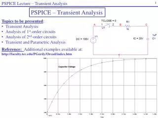
PSPICE Lecture - Transient Analysis 3 Transient Analysis – A transient analysis is used to graph various quantities versus time. Recall that whatever is varied in PSPICE will be placed on the x-axis when graphs are created. So graphs created using a transient analysis will always have time, t, on the x-axis. t = 0 + VR - Example: Use a transient analysis to graph the source voltage, resistor voltage, and capacitor voltage in the circuit below until they reach steady-state. 1 k + VC _ + _ 100 V 1 F
PSPICE Lecture - Transient Analysis 4 Create the Project and draw the circuit: Create a project and draw the circuit shown below. Refer to earlier PSPICE lectures if you need help creating a project. • Notes: • Switch: Use part Sw_tClose from EVAL library for the switch • Nodes: Label the nodes so that they can be referred to when graphing. • Ground: Recall that all analog circuits require the 0 ground.
PSPICE Lecture - Transient Analysis 5 • Initial Capacitor Voltage: You must add the initial capacitor voltage, even if it is 0V. To do this: • Double-click on the capacitor to open the Property Editor (shown on the left below) • Select the part (column) named IC and select the Display tab • Change the Display Format to Name and Value and select OK • IC = should now appear on the schematic. Double-click on it and enter the value (20V in this example)
PSPICE Lecture - Transient Analysis 6 • Capacitor polarity: Capacitors has fixed + and - terminals in PSPICE. This is important when initial conditions are added. The 20V initial condition just added might act like -20V if the capacitor is upside down. To check the polarity: • Select PSPICE – Create Netlist • Select PSPICE – View Netlist • The Netlist shown below indicates that capacitor C1 is connected from node 0 (+) to node C (-), so it is upside down! (The positive node is listed first.) • Right-click on the capacitor and select Mirror Vertically • Check the Netlist to see that the capacitor now has the correct polarity.
PSPICE Lecture - Transient Analysis 7 Create the Simulation Profile: Recall that exponential functions take 5Tau to decay, so we often want to perform a transient analysis for 5Tau. For this example: Length of transient analysis = 5Tau = 5RC = 5(1k)(1uF) = 5ms • Select PSPICE – New Simulation Profile • Give the Simulation Profile a Name (any name is OK but using the schematic name is a good idea) • Under Analysis Type select Time Domain (Transient) • Under Run To Time: Enter 5ms (no spaces!) • Select OK. Fine point: By default approximately 100 points will be used to create each graph, so Maximum step size = (Run to time)/100. In this example the blank box indicates that the Maximum step size is 5ms/100 = 50us. If you wished to use twice as many points you could enter 25us into the Maximum step size box.
PSPICE Lecture - Transient Analysis 8 • Analyze the circuit and graph the results • Select PSPICE – Runto analyze the circuit. The graphing window should appear. Since we did a transient analysis from 0 to 5ms, time should vary from 0 to 5ms on the x-axis.
PSPICE Lecture - Transient Analysis 9 • Add waveforms • Select Trace – Add trace and the Add Traces window will appear. • Select or type the names of one or more waveforms to view • Voltages in the list are all node voltages, so to find the resistor voltage V(B,C) was entered (positive terminal is listed first).
PSPICE Lecture - Transient Analysis Add text Toggle Cursor On/Off Mark Point 10 Add text and mark points Cursor Cursor value – currently for V(B,C) Select Waveform for Cursor
PSPICE Lecture - Transient Analysis 11 • Comments on the graph • Capacitor voltage – Charges from the initial value (20V) to 100V as expected • Resistor voltage – Decays from its initial voltage (100 – 20 = 80V) to zero • Source voltage – Constant 100V
PSPICE Lecture - Transient Analysis 12 • Other graphing features • There are many other graphing features which may be demonstrated in class or you may try on your own. Features include: • Two cursors: PSPICE has two cursors that can be added to determine values of waveforms at different points. • Controlling two cursors: The left-mouse button controls Cursor 1 and the right-mouse button controls Cursor2 (coarse adjustments). The cursors can be moved for fine adjustments with the arrow keys (Cursor1) or Shift + arrow keys (Cursor2). • Marking Points: Use Plot - Label – Markor the toolbar. • Saving graphs: Use Window – Display Control. Last graph is saved here automatically. • Printing graphs: Use Window – Copy to Clipboard. This was used to create the graph on the previous slide. Note that the black background is changed to white. • Graphing expressions: Note the functions in the Add Trace window, such as *, /, abs(), sin(), exp(), etc. You could, for example, graph V(C)*I(C1) or abs(I(C1)). • Trace Properties: Right-click on a trace to change its color, line width, etc. • Other: You can zoom in and out, use linear or log scales, turn off minor gridlines, etc.
PSPICE Lecture - Transient Analysis 13 Charging and discharging a capacitor using VPULSE Suppose that the switch in the circuit below moves back and forth between A and B (for at least 5Tau in each position). The result is that the capacitor will charge and discharge repeatedly. A 1 k + VC _ B + _ VC 100 V 1 F 100 V 0 V Switch moves to A Switch moves to B Switch moves to A Switch moves to B Switch moves to A t 20Tau 5Tau 10Tau 15Tau
PSPICE Lecture - Transient Analysis 14 How is a switch moved back and forth in PSPICE? This is simulated by using a pulse waveform. VPulse Connect 100 V to the RC circuit Connect 0 V to the RC circuit 100 V 0 V t A 20Tau 5Tau 10Tau 15Tau + VC _ + VC _ 1 k 1 k B 0 to100V Pulse Waveform + _ Equivalent circuits 100 V 1 F 1 F
PSPICE Lecture - Transient Analysis 15 Part VPULSE in PSPICE VPULSE is a part in the Source Library. It has various properties as defined below: V1 = First voltage V2 = Second voltage TD = Time Delay (time before pulse starts). It is OK to use TD = 0. TR = Rise Time (time to go from V1 to V2). TR cannot be 0. TF = Fall Time (time to go from V2 to V1). TF cannot be 0. PW = Pulse Width (time when output = V2) PER = Period Illustration: VPulse TF TR V2 PW V1 TD PER t
PSPICE Lecture - Transient Analysis 16 PSPICE Example using part VPULSE
PSPICE Lecture - Transient Analysis 17 Example: Use a transient analysis to graph the capacitor voltage in the circuit below. Assume that the switch moves to position A at t = 0 and then moves back and forth between A and B every 5Tau to repeatedly charge and discharge the capacitor. Graph VC as it charges and discharges 3 times. A + VC _ 1 k B + _ 100 V 1 F
PSPICE Lecture - Transient Analysis 18 Solution: Create the Project and draw the circuit: Create a project and draw the circuit shown below. • Notes: • Use part VPULSE from the Source Library • 5Tau = 5RC = 5ms, so use PW = 5ms (the capacitor charges here) • 5RC is also needed for the capacitor to discharge, so use PER = 10ms (time to charge and discharge) • TR and TF cannot be 0, so make them very small compared to PER. Note that 1ns is only one ten-millionth of PER. • The initial condition for the capacitor must be set to 0V.
PSPICE Lecture - Transient Analysis 19 Create a new Simulation Profile and determine the length of the analysis: In order to charge and discharge the capacitor 3 times, the analysis should last for 30Tau (or 30ms) as illustrated below. VC 100 V 0 V t 30Tau 20Tau 25Tau 5Tau 10Tau 15Tau
PSPICE Lecture - Transient Analysis 20 Simulate the circuit and graph the results:
PSPICE Lecture - Transient Analysis 21 • Parametric Analysis in PSPICE • A parametric analysis is used to vary a second parameter to generate a series of curves. Many types of parametric analysis are possible in PSPICE. • Examples: • Top Example: Vary voltage and current • Bottom Example: Vary time and resistance Vary current (parametric analysis Vary voltage (DC Sweep) Vary R (parametric analysis Vary time (Transient analysis
PSPICE Lecture - Transient Analysis 22 Example: Graph VC versus time as the capacitor charges for R = 10k, 20k, 30k, 40k and 50k. t = 0 R + VC _ + _ 100 V 1 F • Solution: • A transient analysis can be used to vary time from 0 to 5Tau. • Use the largest value of Tau, so 5Tau = 5(50k)(1F) = 250 ms • A parametric analysis can be used to vary R from 10k to 50k
PSPICE Lecture - Transient Analysis 23 Create the Project and draw the circuit: Create a project and draw the circuit shown below. Use the following steps to vary a resistor: Use a variable resistor part, R_var Change the value of R_var to a name in braces, such as {Rvalue} Change the property SET to 1 for R_var (be sure to display it also) Add a part named PARAM from the Special Library Add a property (column) to PARAM with the same name as the resistor value in braces – Rvalue in this cases
PSPICE Lecture - Transient Analysis 24 • Create a new Simulation Profile • Select Time Domain (Transient) for the Analysis type. • Enter 250 ms for the value for Run to time:
PSPICE Lecture - Transient Analysis 25 • Check the box labeled Parametric Sweep. (Note that the window is the same one used with a DC Sweep analysis.) • Select Global parameter • Enter Rvalue for the Parameter name • Enter the Start value, End value, and Increment. • Select OK.
PSPICE Lecture - Transient Analysis Simulate the circuit and graph the results: (Select OK when the Available Sections window appears to select data for all 5 curves.)
PSPICE Lecture - Transient Analysis 27 • Analyzing 2nd-order circuits in PSPICE • There is not much difference betweenanalyzing 2nd-order circuits and analyzing 1st-order circuits. A transient analysis is still used. One difference is in determining the length of the analysis. • 1st-order circuit: • Length of transient analysis = 5Tau • Find Tau = ReqC or L/Req • Or find Tau from the expression x(t) = B + Ae-t/Tau • Example: If v(t) = 10 – 10e-500t, then Tau = 1/500 = 2ms, so 5Tau = 10ms • 2nd-order circuit: • Recall that the natural response has three forms: overdamped, critically-damped, and underdamped. Since an overdamped response has two exponential terms, use the one with the largest Tau (the dominant root). • In each case assume that the exponential terms have the form e-t/Tau and again use: Length of transient analysis = 5Tau • Example: If v(t) = e-500t[20cos(50t) + 30sin(50t)] (underdamped), then Tau = 1/500 = 2ms, so 5Tau = 10ms
PSPICE Lecture - Transient Analysis 28 Example: Graph VC versus time until the capacitor reaches steady state. t = 0 1 mH 12.62 + VC _ + _ 20 V 1.57 F Solution:First determine the length of the analysis. This is a series RLC circuit so:
PSPICE Lecture - Transient Analysis 29 Create the Project and draw the circuit: Create a project and draw the circuit shown below. • Notes: • Set the initial condition to 0 for the capacitor and the inductor (IC = 0). • Label the nodes. The node voltage V(C) is the capacitor voltage. • Create the simulation profile • Perform a transient analysis from 0 to 0.8 ms • 3. Analyze the circuit and graph the capacitor voltage • See the following slide
PSPICE Lecture - Transient Analysis 30 Note that the capacitor voltage is as expected: It has an initial voltage of 0V, a final voltage of 20V, and it is underdamped. Two other quantities are useful to show on this graph: rise time and % overshoot. They are defined on the following slides.
PSPICE Lecture - Transient Analysis 31 Rise Time(tr) – the time for a waveform to go from 10% of its final value to 90% of its final value. Rise time can be used with any order circuit and any type of response. Example: 10V 9V 1V tr t 0V
PSPICE Lecture - Transient Analysis 32 % Overshoot – This term is only used with underdampedcircuits. It is a measure of how far the waveform shoots past its final value before settling on the final value. It is defined (for a voltage) as: Example: v(t) 13V 10V 0V t
PSPICE Lecture - Transient Analysis 33 Add rise time and % overshoot to the previous graph: • A cursor was used to mark 3 points at: • 2V (10% of the 20V final value) • 18V (90% of the 20V final value) • The max value (use the cursor peak tool)