Credit Risk
Credit Risk. Yiling Lai 2008/10/3. Outline. Introduction Credit Ratings Historical Default Probabilities Recovery Rates Estimating Default Probability from Bond Prices Comparison of Default Probability Estimates. Introduction.

Credit Risk
E N D
Presentation Transcript
Credit Risk Yiling Lai 2008/10/3
Outline • Introduction • Credit Ratings • Historical Default Probabilities • Recovery Rates • Estimating Default Probability from Bond Prices • Comparison of Default Probability Estimates
Introduction • Credit risk raises from the possibility that borrowers and counterparties in derivatives transactions may default.
Credit Rating • Credit Rating assesses the creditworthiness of corporate bonds. Investment grade bond Non-investment grade bond (high yield bond, speculative grade bond or junk bond)
Historical Default Probabilities • Average cumulative default rates(%), 1970-2006. Source: Moody’s • From this table, we can calculate unconditional default probability and conditional default probability.
Historical Default Probabilities • Unconditional default probability • The probability of a bond defaulting during a particular year as seen at time 0. Increasing 0.352 =0.506-0.181 Decreasing
Historical Default Probabilities • Conditional default probability (default intensity or hazard rate) • The probability that the bond will default during a particular year conditional on no earlier default. The probability that the bond will survive until the end of year 2 is 100-30.949=69.506% Conditional default probability is 9.223/69.506 = 13.27% (for 1-year time period)
Default Intensities • Q(t): the probability of default by time t.
Recovery Rates • The recovery rate for a bond is normally defined as the bond’s market value immediately after a default, as a percent of its face value.
Recovery Rates • Recovery rates are significantly negatively correlated with default rates. • Recovery rate = 59.1 - 8.356 x Default rate • The recovery rate: the average recovery rate on senior unsecured bonds in a year measured as % • The default rate: the corporate default rate in the year measured as % • A bad year for the default rate is usually double bad because it is accompanied by a low recovery rate. Default rate = 0.1% => Recovery rate = 58.3% Default rate = 3% => Recovery rate = 34.0%
Estimating Default Probability from Bond Prices • Assumption: The only reason a corporate bond sells for less than a similar risk-free bond is the possibility default. • An approximate calculation: S = 200 base points and R = 40% => h=0.02/(1-0.4)=3.33%
A More Exact Calculation • The corporate bond: • Period: 5 years • Coupon: 6% per annum (paid semiannually) • Yield: 7% per annum (with continuous compounding) • Price: 95.34 • A similar risk-free bond • Yield: 5% per annum (with continuous compounding) • Price: 104.09 • The expected loss from default over the 5-year life of the bond is 104.9-95.34=$8.75
A More Exact Calculation • Assumption: defaults can happen at times 0.5, 1.5, 2.5, 3.5, and 4.5 years (immediately before coupon payment dates). • Notional Principal=$100 • Risk-free rates: 5% (with continuous compounding) • Recovery rate = 40% => 100*40%=$40
A More Exact Calculation • Consider the 3.5 years: • The expected value of the risk-free bond at time 3.5 years: • The loss given default is 104.34-40=64.34 • The PV of this loss is years 0 1 2 3 4 5 Cash flow 3 3 3 103
A More Exact Calculation • Suppose that the probability of default per year (assumed to be the same each year) is Q. • Calculating of loss from default on a bond in terms of the default probabilities per year, Q. 288.48Q=8.75 => Q = 3.03%
A More Exact Calculation • We can extend this calculations by changing some assumptions. • Example: • Defaults can take place more frequently • A constant default intensity • A particular pattern for the variation of default probabilities with time • With several bonds we can estimate several parameters describing the term structure of default probabilities.
The Risk-Free Rate • The benchmark risk-free rate that is usually used in quoting corporate bond yields is the yield on similar Treasury bonds. • In fact, those derivative traders usually use LIBOR rates as short-term risk-free rates. • They regard LIBOR as their opportunity cost of capital. • Treasury rates are too low to be used as risk-free rates.
Asset Swaps • Asset swaps = asset + interest rate swap or Asset swaps = asset + currency swap • An asset swap transforms the character of an end user’s assets. • Repacking an issue paying fixed rates into floating rates (or vice versa) • Converting cash flow stated in one currency to another. • It does not eliminate the asset from an investor’s portfolio.
Fixed Rates to Floating Rates • The investor transforms the yield on its fixed rate asset into a floating rate asset.
Currency Transformation • The investor converts with the swap counterparty the FFr500mm principal cost of the asset and $100mm, the investor’s base currency.
Asset Swaps Spread • In practice, traders often use asset swap spreads as a way of extracting default probabilities from bond prices. • Asset swap spreads provide a direct estimate of the spread of bond yields over the LIBOR/swap curve. • Example: • An asset swap spread for a particular bond: 150 bps • The LIBOR/swap zero curve is flat at 5% • The amount by which the value of the risk-free bond exceeds the value of the corporate is the present value of 150bps per year for 5years. • Assuming semiannual payments
Asset Swaps Spread • The sum of PV is $6.55 per $100 of principal. • 288.48Q = 6.55 => Q=2.27% years 0 1 2 3 4 5 Cash flow 0.75 0.75 0.75 0.75 0.75 0.75 0.75 0.75 0.75 0.75 PV
Comparison of Default Probability Estimates (part I) • From historical data: • Based on • Consider t=7: • Consider an A-rated company in table 20.1: Q(7) =0.00759
Comparison of Default Probability Estimates (part I) • From bond prices: • Based on • Recovery rate (R): 40% • Risk-free rate: the 7-year swap rate minus 10 bps. • For A-rated bond, the average Merrill Lynch yield was 5.993% • The average swap rate was 5.398% => risk-free rate = 5.398-0.1=5.298% s = 0.05993-0.05298 = 0.00695
Comparison of Default Probability Estimates (part I) increase decline
Comparison of Default Probability Estimates (part II) • Another way of looking at these results: excess return over the risk-free rate increase Historicaldefault intensity x (1-Recovery rate)
Real-World vs. Risk-Neutral Probabilities • The default probabilities implied from bond yields are risk-neutral probabilities of default. • The risk-neutral valuation principle states that the price of a derivative is given by the expectation of the discounted terminal payoff under the risk neutral measure. • This means that the default probability Q must be a risk-neutral probability. • By contrast, the default probabilities implied from historical data are real-world probabilities of default.
Why do we see such big differences between real-world and risk-neutral default probabilities? • Corporate bonds are relatively illiquid. • The subjective default probabilities of bond traders may be much higher than those given in Tables 20.1. • Bonds do not default independently of each other because of systematic risk. • Unsystematic risk: It is much more difficult to diversify risks in a bond portfolio than in an equity portfolio.
Which one is better? • The answer depends on the purpose of the analysis. • Risk-neutral default probabilities: • To value credit derivatives • To estimate the impact of default risk • Real-world default probabilities: • To calculate potential future losses from default when carrying out scenario analyses

