EEET 5101 Information Theory Chapter 1
EEET 5101 Information Theory Chapter 1. Introduction Probability Theory. BY Wai (W2-4) siuwai.ho@unisa.edu.au. Basic Course Information. Lecturers: Dr Siu Wai Ho, W2-4, Mawson Lakes Dr Badri Vellambi Ravisankar, W1-22, Mawson Lakes Dr Roy Timo, W1-7, Mawson Lakes

EEET 5101 Information Theory Chapter 1
E N D
Presentation Transcript
EEET 5101 Information TheoryChapter 1 Introduction Probability Theory BY Wai (W2-4) siuwai.ho@unisa.edu.au
Basic Course Information • Lecturers: • Dr Siu Wai Ho, W2-4, Mawson Lakes • Dr Badri Vellambi Ravisankar, W1-22, Mawson Lakes • Dr Roy Timo, W1-7, Mawson Lakes • Office Hour: Tue 2:00-5:00pm (starting from 27/7/2010) • Class workload: • Homework Assignment 25% • Mid-term 25% • Final 50% • Textbook: T. M. Cover and J. M. Thomas, Elements of Information Theory, 2nd, Wiley-Interscience, 2006.
Basic Course Information • References: • OTHER RELEVANT TEXTS (Library): • 1. Information Theory and Network Coding by Raymond Yeung • 2. Information Theory: Coding Theorems for Discrete Memoryless Systems by Imre Csiszar and Janos Korner. • OTHER RELEVANT TEXTS (Online): • 3. Probability, Random Processes, and Ergodic Properties by Robert Gray • 4. Introduction to Statistical Signal Processing Robert Gray and L. Davisson • 5. Entropy and Information Theory by Robert Gray http://ee.stanford.edu/~gray/
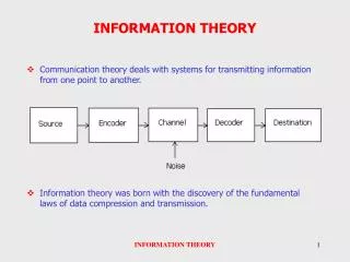
The Beginning of Information Theory • In 1948, Claude E. Shannon published his paper “A Mathematical Theory of Communication” in the Bell Systems Technical Journal. • He introduced two fundamental concepts about “information”: • Information can be measured by entropy • Information to be transmitted is digital Information Source Transmitter Receiver Destination Received Signal Signal Message Message Noise Source
The Beginning of Information Theory • In the same paper, he has answered two fundamental questions in communication theory: • What is the ultimate data compression ? • How to minimize the compression rate m/n with Pr{uv} = 0. • What is the ultimate transmission rate of communication? • How to maximize the transmission rate n/m with Pr{kk’} 0. u = u1 … un x1 … xm v = v1 … vn Source Receiver Encoder Decoder x1 … xm y1 … ym k {1,…,2n} k’ Source Receiver Encoder Channel Decoder
The Idea of Channel Capacity • Example [MacKay 2003]: Suppose we are now provided a noisy channel • We test it 10000 times and find the following statistics • Pr{y=0|x=0} = Pr{y=1|x=1} = 0.9; Pr{y=0|x=1} = Pr{y=1|x=0} = 0.1 • The occurrence of difference is independent of the previous use • Suppose we want to send a message: s = 0 0 1 0 1 1 0 • The error probability = 1 – Pr{no error} = 1 – 0.97 0.5217 • How can we get a smaller error probability? x Channel y 0.9 0 0 0.1 1 1 0.9
The Idea of Channel Capacity • Method 1: Repetition codes • [R3] To replace the source message by 0 000; 1 111 • The original bit error probability Pb : 0.1. The new Pb : = 3 0.9 0.12 + 0.13 = 0.028 • bit error probability 0 rate 0 ?? t: transmitted symbols n: noise r: received symbols Majority voteat the receiver
The Idea of Channel Capacity • Method 1: Repetition codes pb 0 rate 0
The Idea of Channel Capacity • Method 2: Hamming codes • [(7,4) Hamming Code] group 4 bits into s. E.g., s = 0 0 1 0 • Here t = GTs = 0 0 1 0 1 1 1, where
The Idea of Channel Capacity • Method 2: Hamming codes • Is the search of a good code an everlasting job? Where is the destination?
The Idea of Channel Capacity • Information theory tells us the fundamental limits. • It is impossible to design a code with coding rate and error probability on the right side of the line. Shannon’ s Channel Coding Theorem
Intersections with other Fields • Information theory showsthe fundamental limits indifferent communicationsystems • It also provides insightson how to achieve these limits • It also intersects other fields[Cover and Thomas 2006]
Content in this course • 2) Information Measures and Divergence: • 2a) Entropy, Mutual Information and Kullback-Leibler Divergence -Definitions, chain rules, relations • 2b) Basic Lemmas & Inequalities: -Data Processing Inequality, Fano’s Inequality. • 3) Asymptotic Equipartition Property (AEP) for iid Random Processes: • 3a) Weak Law of Large Numbers • 3b) AEP as a consequence of the Weak Law of Large Numbers • 3c) Tail event bounding: -Markov, Chebychev and Chernoff bounds • 3d) Types and Typicality -Strong and weak typicality • 3e) The lossless source coding theorem
Content in this course • 4) The AEP for Non-iid Random Processes: • 4a) Random Processes with memory -Markov processes, stationarity and ergodicity • 4b) Entropy Rate • 4c) The lossless source coding theorem • 5) Lossy Compression: • 5a) Motivation • 5b) Rate-distortion (RD) theory for DMSs (Coding and Converse theorems). • 5c) Computation of the RD function (numerical and analytical) • How to minimize the compression rate m/n with uand v satisfying certain distortion criteria. u = u1 … un x1 … xm v = v1 … vn Source Receiver Encoder Decoder
Content in this course • 6) Reliable Communication over Noisy Channels: • 6a) Discrete memoryless channels -Codes, rates, redundancy and reliable communication • 6b) Shannon’s channel coding theorem and its converse • 6c) Computation of channel capacity (numerical and analytical) • 6d) Joint source-channel coding and the principle of separation • 6e) Dualities between channel capacity and rate-distortion theory • 6f) Extensions of Shannon’s capacity to channels with memory (if time permits)
Content in this course • 7) Lossy Source Coding and Channel Coding with Side-Information: • 7a) Rate Distortion with Side Information -Joint and conditional rate-distortion theory, Wyner-Ziv coding, extended Shannon lower bound, numerical computation • 7b) Channel Capacity with Side Information • 7c) Dualities • 8) Introduction to Multi-User Information Theory (If time permits): • Possible topics: lossless and lossy distributed source coding, multiple access channels, broadcast channels, interference channels, multiple descriptions, successive refinement of information, and the failure of source-channel separation.
Prerequisites – Probability Theory • LetX be a discrete random variable taking values from the alphabet • The probability distribution of X is denoted by pX = {pX(x), xX}, where • pX(x) means the probability that X = x. • pX(x) 0 • xpX(x) = 1 • Let SX be the support of X, i.e. SX = {xX: p(x) > 0}. • Example : • Let X be the outcome of a dice • Let = {1, 2, 3, 4, 5, 6, 7, 8, 9, …} equal to all positive integers.In this case, is a countably infinite alphabet • SX = {1, 2, 3, 4, 5, 6} which is a finite alphabet • If the dice is fair, then pX(1) = pX(2) = = pX(6) = 1/6. • If is a subset of real numbers, e.g., = [0, 1], is a continuous alphabet and X is a continuous random variable
Prerequisites – Probability Theory • Let X and Y be random variable taking values from the alphabet Xand Y, respectively • The joint probability distribution of X and Y is denoted by pXY and • pXY(xy) means the probability that X = xand Y = y • pX(x), pY(y), pXY(xy) p(x), p(y), p(xy) when there is no ambiguity. • pXY(x) 0 • xypXY(x) = 1 • Marginal distributions: pX(x) = ypXY(xy) and pY(y) = xpXY(xy) • Conditional probability: for pX(x) > 0, pY|X(y|x) = pXY(xy)/ pX(x) which denotes the probability that Y = y given the conditional that X = x • Consider a function f: XY • If X is a random variable, f(X) is also random. Let Y = f(X). • E.g., X is the outcome of a fair dice and f(X) = (X – 3.5)2 • What is pXY? X PY|X Y
Expectation and Variance • The expectation of X is given by E[X] = xpX(x) x • The variance of X is given by E[(X – E[X])2] = E[X2] – (E[X])2 • The expected value of f(X) is E[f(X)] = xpX(x) f(x) • The expected value of k(X, Y) is E[k(X, Y)] = xypXY(xy) k(x,y) • We can take the expectation on only Y, i.e., EY[k(X, Y)] = ypY(y) k(X,y) which is still a random variable • E.g., Suppose some real-valued functions f, g, k and l are given. • What is E[f(X, g(Y), k(X,Y))l(Y)]? • xypXY(xy) f(x, g(y), k(x,y))l(y) which gives a real value • What is EY[f(X, g(Y), k(X,Y)]l(Y)? • ypY(y) f(X, g(y), k(X,y))l(y) which is still a random variable. • Usually, this can be done only if X and Y are independent.
Conditional Independent • Two r.v. X and Y are independent if p(xy) = p(x)p(y) x, y • For r.v. X, Y and Z, X and Z are independent conditioning on Y, denoted by X Z | Yif p(xyz)p(y) = p(xy)p(yz) x, y, z ----- (1) • Assume p(y) > 0, p(x, z|y) = p(x|y)p(z|y) x, y, z ----- (2) • If (1) is true, then (2) is also true given p(y) > 0 • If p(y) = 0, p(x, z|y) may be undefined for a given p(x, y, z). • Regardless whether p(y) = 0 for some y, (1) is a sufficient condition to test X Z | Y • p(xy) = p(x)p(y) is also called pairwise independent
Mutual and Pairwise Independent • Mutual Indep.:p(x1, x2, …, xn) = p(x1)p(x2) p(xn) • Mutual IndependentPairwise Independent • Suppose we have i, j s.t. i, j [1, n] and i j • Let a = [1, n] \ {i, j} • Pairwise IndependentMutual Independent
Mutual and Pairwise Independent • Example :Z = XY and Pr{X=0} = Pr{X=1} = Pr{Y=0} = Pr{Y=1} = 0.5 • Pr{Z=0} = Pr{X=0}Pr{Y=0} + Pr{X=1}Pr{Y=1} = 0.5 • Pr{Z=1} = 0.5 • Pr{X=0, Y=0} = 0.25 = Pr{X=0}Pr{Y=0} • Pr{X=0, Z=1} = 0.25 = Pr{X=0}Pr{Z=1} • Pr{Y=1, Z=1} = 0.25 = Pr{Y=1}Pr{Z=1} …….. • So X, Y and Z are pairwise Independent • However, Pr{X=0, Y=0, Z=0} = Pr{X=0}Pr{Y=0} = 0.25 • Pr{X=0}Pr{Y=0}Pr{Z=0} = 0.125 • X, Yand Z are not mutually Independent but pairwise Independent