(from halliburton)
Optimization of Advanced Well Type and Performance Louis J. Durlofsky. (from www.halliburton.com). Department of Petroleum Engineering, Stanford University ChevronTexaco ETC, San Ramon, CA. Acknowledgments. B. Yeten, I. Aitokhuehi, V. Artus K. Aziz, P. Sarma. Multilateral Well Types.

(from halliburton)
E N D
Presentation Transcript
Optimization of Advanced Well Type and Performance Louis J. Durlofsky (from www.halliburton.com) Department of Petroleum Engineering, Stanford University ChevronTexaco ETC, San Ramon, CA
Acknowledgments • B. Yeten, I. Aitokhuehi, V. Artus • K. Aziz, P. Sarma
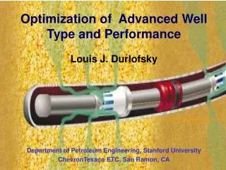
Multilateral Well Types TAML, 1999
Optimization of NCW Type and Placement • Applying a Genetic Algorithm that optimizes via analogy to Darwinian natural selection • GA approach combines “survival of the fittest” with stochastic information exchange • Algorithm includes populations with generations that reproduce with crossover and mutation • General level of fitness as well as most fit individual tend to increase as algorithm proceeds
101011011010110101111101100010110011010011010... I1 J1 K1 lxyq hz Jn lxyq hz heel heel toe toe main trunk lateral multilateral well Encoding of Unknowns for GA • Representation allows well type to evolve (Jn 0 generates a lateral)
Nonconventional Well Optimization Unknowns Objective Function • Objective function can be any simulation output (NPV, cumulative oil)
Flowchart for Single Geological Model Objective function f (or fitness): NPV, cumulative oil
Single Well Optimization Example • Objective: optimum well and production rate that maximizes NPV, subject to GOR, WOR constraints Optimum well (quad-lateral) (from Yeten et al., 2003)
Evolution of Well Types (from Yeten et al., 2003)
Nonconventional Well Optimization with Geological Uncertainty ?
i Optimization over Multiple Realizations • Find well that maximizes F = < f > + r s ( < f > is average fitness of well over N realizations, r is risk attitude, s2is variance in f over realizations) • Evaluate each individual (well) for each realization (well i, realization j)
Risk Neutral (r =0) Optimization(Primary Production, Maximize NPV) NPV ($) Realization #
Risk Averse (r = -0.5) Optimization(Primary Production, Maximize NPV) NPV ($) Realization #
Comparison of Optimization Results Risk neutral attitude (r = 0) well cost = $ 759,158 expected NPV = $ 3,506,390 std = $ 935,720 NPV ($) Risk averse attitude (r = -0.5) well cost = $ 1,058,704 expected NPV = $ 3,401,210 std = $ 404,920 Realization #
attribute 1 attribute 1 attribute 2 attribute 2 fitness cluster # Proxy - Unsupervised Cluster Analysis • Attributes can be combined into principal components
r = 0.93 estimated fitness actual fitness Proxy Estimate for a Single Realization(Primary Production, Monobore Wells)
r = 0.97 estimated mean fitness actual mean fitness Estimated Mean for All Realization(Primary Production, Monobore Wells)
Smart Well Control: “Reactive” versus “Defensive” • Reactive control: adjust downhole settings to react to problems (e.g., water or gas production) as they occur • Defensive control: optimize downhole settings to avoid or minimize problems. This requires: • Accurate reservoir description (HM models) • Optimization procedure • Optimize using gradients computed numerically or via adjoint procedure
Numerical Gradients • Define cost function J (NPV, cumulative oil) x - dynamical states, u - controls • Numerically compute J/u • Apply conjugate gradient technique to drive J/u to 0
Adjoint Procedure • Define augmented cost function JA l- Lagrange multipliers, x - dynamical states, u - controls, g - reservoir simulation equations • Optimality requires first variation of JA= 0 (dJA= 0): adjoint equations optimality criteria
Adjoint versus Numerical Gradient Approaches for Optimization • Numerical Gradients • Advantages • Easily implemented • No simulator source code required • Main Drawback • CPU requirements • Adjoint Gradients • Advantages • Much faster for large number of wells & updates • Can also be used for HM • Main Drawback • Adjoint simulator required • Adjoint and numerical gradient procedures developed; implementation of smart well model into GPRS underway
Smart Well Model • Numerical gradient approach (Yeten et al., 2002) allows use of existing (commercial) simulator • ApplyingECLIPSEmulti-segment wells option
Optimization Methodology - Fixed Geology • Sequential restarts applied to determine optimal settings
Impact of Smart Well Control - Example • Channelized reservoir, 4 controlled branches • Production at fixed liquid rate with GOR and WOR constraints (three-phase system)
Effect of Valve Control on Oil Production Oil rate - uncontrolled case Oil rate - controlled case • Downhole control provides an increase in cumulative oil production of 47% (from Yeten et al., 2002)
Optimization with History Matching • Actual geology is unknown (one model selected randomly represents “actual” reservoir and provides “production” data) • Update reservoir models based on synthetic history • Optimize using current (history-matched) model
History Matching Procedure • Facies-based probability perturbation algorithms (Caers, 2003) • Multiple-point geostatistics (training images) • Performs two levels of nonlinear optimization (facies and k-f) • History matching based on well pressure, cumulative oil and water cut (for each branch) • Initial models from same training image as “actual” models
History Matching Objective Functions • Two levels of optimization • Single parameter facies optimization • Multivariate permeability-porosity optimization
Channelized Model I • Unconditioned 2 facies model, 20 x 20 x 6 grid • Quad-lateral well with a valve on each branch • Constant total fluid rate (10 MSTB/D initial liquid rate) • Shut-in well if water cut > 80% • OWG flow, M < 1; 4 optimization and HM steps
Optimization on Known Geology • Valves provide ~40% gain in cumulative oil over no-valve base case
Dimensionless Increase in Np • Dimensionless cumulative oil difference, N N = 0 (no valves result) N = 1 (known geology result)
DN =1 DN =0.5 DN =0 Illustration of Incremental Recovery HM with valves
Optimization with History Matching • Optimization with history matching gives N=0.94 • Repeating for different initial models: N=0.900.18
Channelized Model II • Unconditioned 2 facies model, 20 x 20 x 6 grid • Different training image than Channelized Model I, same well and other system parameters
DN =0.41 Optimization with History Matching - CM II • Repeating for different initial models: N=0.440.27 • Inaccuracy may be due to nonuniqueness of HM
Optimization over Multiple HM Models Number of HM Models DN (s) 1 0.44 0.27 3 0.85 0.16 5 0.84 • Use of multiple history-matched models provides significant gains
Effect of Conditioning (on Facies) Single HM Model • Partial redundancy of conditioning and production data reduces impact of conditioning in some cases • For CM II, use of 3 conditioned and history matched models gives DN = 0.83 0.10 (~same as w/o cond)
Summary • Presented genetic algorithm for optimization of nonconventional well type and placement • Applied GA under geological uncertainty • Developed combined valve optimization – history matching procedure for real-time smart well control • Demonstrated that optimization over multiple history-matched models beneficial in some cases
Research Directions • Developing efficient proxies for optimization of well type and placement under geological uncertainty • Implementing adjoint approach (optimal control theory) and multisegment well model into GPRS for determination of valve settings • Plan to incorporate additional data (4D seismic) and accelerate history matching procedure