Download
1 / 65
1.08k likes | 1.99k Vues
The Four-Step Travel Model . GEOG 111 & 211A – Fall 2006. Outline. Background Role of Simulation General Process Example of Most Popular Simulation Model Examples of Other Ideas Summary. Needs. Identify Projects for the Region

E N D
The Four-Step Travel Model GEOG 111 & 211A – Fall 2006
Outline • Background • Role of Simulation • General Process • Example of Most Popular Simulation Model • Examples of Other Ideas • Summary
Needs • Identify Projects for the Region • Use Formal & Accepted Technique(s) to Estimate Project Impacts • Simulate the Region for the Next 20 Years • Create Scenarios for BEFORE and AFTER a Project or Group of Projects
How Do we use Simulation Models? • Create a Comprehensive Plan of how we want an area/region to be in the future • Propose projects designed to achieve the goals of the Comprehensive Plan • Test Scenarios implementing different projects and forecast their effects • Determine what projects should be continued to next stage • Present recommendations to decision makers
Project Types • New Highways (e.g., bypass-ring roads) • New Management Activities (e.g., park & ride, signal systems ) • New Land Uses (e.g., a new industry, a new residential neighborhood) • New Technologies??????? (maybe in management)
The Context • Urban Transportation Planning System (UTPS) & Urban Transportation Modeling System • TEA 21 made it also A Statewide Transportation Planning System • Technology should be added (see Pennplan) • Associate quantitative estimates with performance measures as in the monitoring part (see PennPlan) • Four-step scheme followed today in many MPOs • Four-step travel model is limited but popular!
Goals and objectives Calibrate models Land use Trip generation Trip distribution Modal split Traffic assign. Analysis of future alternative systems Inventories and data collection Transportation organizations Develop alternatives Apply models Land use Trip generation Trip distribution Mode choice Traffic assign. Plan testing, evaluation and selection Population Land use Economic activity Transportation system Travel volumes Terminal and transfer facilities status & use Financial resources Community values D A T A PennDOT MPOs TMAs LDDs Local gov’ts Citizen participation Areawide forecast Population Land use Economic Traffic Revenues Policy and technical development Continuing elements Plan implementation Develop immediate action plan Surveillance Reappraisal Procedural development Service Annual report = Part of the Sequential Demand Forecasting Process Typical Process in Long Range Planning
Land use and socioeconomic projections Direct (user) Impacts Trip Generation The Sequential Forecasting Process & the Urban Transportation Planning System (UTPS)[adapted from Papacostas & Prevedouros, 1993] 4 - S T E P Trip Distribution Transportation system specification Mode Choice Network Assignment
Four step in large MPOs • Inventory of facilities • Opportunity to think strategically • Show the impact of projects on air quality • Provide report of emissions inventory • Tool for policy assessment • PSRC example follows!
What Other Steps Are Required? • Forecast future development (business, roadways, and housing) • Model the area’s traffic network • Estimate model of the area’s traffic network in the future • Make changes to network characteristics in the future model • Compare network performance under different scenarios of project development
UTPS Outline • Review the Data Inventory for a Region • Review one Procedure to Predict Future Volumes on a Highway • Summarize the Method Known as UTPS • Questions
UTPS 4-step Travel Model • Trip Generation • Trip Distribution • Modal Split • Traffic Assignment
Data (Inventory) • Area of study definition & traffic analysis zones • Area of study description (highways, facilities, zoning, rules/regulations) • Who are the residents? (age, gender, education, employment, income of residents) • Where do people leave? • Where do people work, shop, etc? • Highway characteristics • Other information (plans for rezoning)
Travel Model • Urban Travel Model (‘60s) • Also known as the Four - Step Process • A methodology to model traffic on a network • General planning & programming • Land use forecasting (where will residences and stores be?) • Four Steps: • Trip Generation Estimate Person Trips for each TAZ • Trip Distribution Distribute Person Trips from TAZ to TAZ • Mode Choice Convert Person Trips to Vehicle Trips • Traffic Assignment Assign Vehicles to the Network
Key Concepts of 4-step Block Block Group Tract i.e., a city block • TAZ: Traffic Analysis Zone • TAZ= a common sense subdivision of the study area • TAZs are used in trip generation and trip distribution • TAZs may be any shape or size, but US Census Blocks, Block Groups, and Tracts are often used (class: WHY?)
x study area boundary = TAZ designations TAZ boundaries 8-Zone Study Area 2 3 1 8-Zone Study Area with Traffic Analysis Zones (TAZs) 5 z 4 8 6 7 Legend: z = all zones outside study area
Key Concepts of UTPS • Centroid • Every TAZ (Gate and Internal) has a centroid, usually placed roughly at the geographic center of the TAZ • All trips to or from a TAZ are assumed to start or end at the centroid • Discussion • Why do we use TAZs and centroids to model trips?
Key Concepts of UTPS • Gate TAZs • TAZs placed outside the Study Area where major roads cross the boundaries of the study area • Used to model External Trips (i.e., trips with an origin or destination) Note: Do we care when OD is outside the study area? • Gate TAZs represent all areas outside of the study area Network Gate TAZ (Study Area)
Example: Computer schematic representation Network & Links Numbered 22 23 20 21 18 19 16 17 13 14 15 8 9 10 11 12 5 6 7 3 4 2 1
Network and Nodes Numbered 23 22 19 20 21 14 15 16 17 18 8 9 10 11 12 13 3 4 5 6 7 2 1
Centroid Gate TAZ
Land Use/Economic Analysis • Considers general trends • Allocates population to geographic subdivisions • Assigns land uses • Each TAZ contains “observed” numbers for today’s analysis and predicted numbers for forecasting
OUTPUT = a map with TAZ’s and their characteristics – households, businesses, employers
Trip Generation Process • Collect Data, usually by Surveys and Census • Sociodemographic Data and Travel Behavior Data • Create a Trip Generation Model (e.g., regression) • Estimate the number of Productions and Attractions for each TAZ, by Trip Purpose • Balance Productions and Attractions for each Trip Purpose • Total number of Productions and Attractions must be equal for each Trip Purpose • We will discuss balancing later
Trip Generation Models • Regression Models • Explanatory Variables are used to predict trip generation rates, usually by Multiple Regression • Trip Rate Analysis • Average trip generation rates are associated with different trip generators or land uses • Cross - Classification / Category Analysis • Average trip generation rates are associated with different trip generators or land uses as a function of generator or land use attributes • Models may be TAZ, Household, or Person - Based
ITE Trip Generation Manual • Trip Rate Analysis Model • Univariate regression for trip generation • Primarily for Businesses • Explanatory variables are usually number of employees or square footage • Models developed using data from national averages and numerous studies from around the US
Possible geographic detail in trip generation with GIS & business data
OUTPUT Typical output from trip generation
Trip Distribution Destinations TAZ P 15 13 26 18 8 13 93 A 22 6 5 52 2 6 93 Origins 1 2 3 4 5 6 Sum T11 T12 T13 T14 T15 T16 O1 T21 T22 T23 T24 T25 T26 O2 T31 T32 T33 T34 T35 T36 O3 T41 T42 T43 T44 T45 T46 O4 T51 T52 T53 T54 T55 T56 O5 T61 T62 T63 T64 T65 T66 O6 D1 D2 D3 D4 D5 D6 1 2 3 4 5 6 Sum 1 2 3 4 5 6 Sum • Convert Production and Attraction Tables into Origin - Destination (O - D) Matrices
Trip Distribution, Methodology • General Equation: • Tij = Ti P(Tj) • Tij = calculated trips from zone i to zone j • Ti = total trips originating at zone i • P(Tj) = probability measure that trips will be attracted to zone j • Constraints: • Singly Constrained • Sumi Tij = Dj OR Sumj Tij = Oi • Doubly Constrained • Sumi Tij = Dj AND Sumj Tij = Oi
Trip Distribution Models Example • Gravity Model Tij is: • Tij = trips from zone i to zone j = • Ti = total trips originating at zone i • Aj = attraction factor at j • Ax = attraction factor at any zone x • Cij = travel friction from i to j expressed as a generalized cost function • Cix = travel friction from i to any zone x expressed as a generalized cost function • a = friction exponent or restraining influence a TiAj / Cij a Sum (Ax / Cix)
Gravity Model Process • Create Shortest Path Matrix • How: Minimize Link Cost among Centroids • Estimate Friction Factor Parameters • How: Function of Trip Length Characteristics by Trip Purpose • Calculate Friction Factor Matrix • Convert Productions and Attractions to Origins and Destinations • Calculate Origin - Destination Matrix • Enforce Constraints on O - D Matrix
Shortest Path Matrix • Matrix of Minimum Generalized Cost from any Zone i to any Zone j • Distance, Time, Monetary Cost, Waiting Time, Transfer Time, etc.. may be used in Generalized Cost • Time or Distance Often Used • Matrix Not Necessarily Symmetric (Effect of One - Way Streets) TAZ ID TAZ ID 1 2 3 4 5 6 C11 C12 C13 C14 C15 C16 C21 C22 C23 C24 C25 C26 C31 C32 C33 C34 C35 C36 C41 C42 C43 C44 C45 C46 C51 C52 C53 C54 C55 C56 C61 C62 C63 C64 C65 C66 1 2 3 4 5 6
O - D Matrix Calculation • Calculate Initial Matrix By Gravity Equation, by Trip Purpose • Each Cell has a Different Friction, Found in the Corresponding Cell of the Friction Factor Matrix • Enforce Constraints in Iterative Process • Sum of Trips in Row i Must Equal Origins of TAZ i • Sum of Trips in Column j Must Equal Destinations of TAZ j • Iterate Until No Adjustments Required
O - D Matrix Example: Destinations Origins 1 2 3 4 5 6 Sum T11 T12 T13 T14 T15 T16 O1 T21 T22 T23 T24 T25 T26 O2 T31 T32 T33 T34 T35 T36 O3 T41 T42 T43 T44 T45 T46 O4 T51 T52 T53 T54 T55 T56 O5 T61 T62 T63 T64 T65 T66 O6 D1 D2 D3 D4 D5 D6 1 2 3 4 5 6 Sum
Final O - D Matrix • Combine (Add) O - D Matrices for Various Trip Purposes • Scale Matrix for Peak Hour • Scale by Percent of Daily Trips Made in the Peak Hour • 0.1 Often Used • Scale Matrix for Vehicle Trips • Scale by Inverse of Ridership Ratio to Convert Person Trips to Vehicle Trips • 0.95 to 1 Often Used • Note: Other Mode Split Process / Models using Discrete Choice may be More Accurate
OUTPUT = the trip interchange matrix and the shortest path trees
Modal Split • Use a model to convert trips into vehicle trips • Usually public transportation versus private car • Nomographs, Regression methods, Microeconomic Regression methods • Stated Preference (conjoint measurement) techniques for hypothetical options • Traveler objective and subjective constraints in selecting a mode
OUTPUT = a trip interchange matrix for each mode: car, public transportation, could also be pedestrian but not usual
Traffic Assignment • Fourth Step in UTPS Modeling • Inputs: • Peak Hour, Passenger Vehicle Origin - Destination (O - D) Matrix • Network • Travel Time, Capacity, Direction • Outputs: • Peak Hour Volumes, Estimated Travel Times, and Volume to Capacity Ratios
Roadway Performance Functions • Traffic Flow and Travel Time Linear Relationship Non-Linear Relationship Route Travel Time Capacity Free-Flow Travel Time Traffic Flow Traffic Flow
Assignment Methods • All or Nothing • All traffic from zone i to zone j uses the (initially) minimal travel time path • Roadway performance not used • System Equilibrium • Assignment is performed such that total system travel time is minimized (UPS, Fed-EX).
Assignment Methods • User Equilibrium • Travel time from zone i to zone j cannot be decreased by using an alternate route • Roadway performance used • Stochastic User Equilibrium • Same as User Equilibrium but accounts for user variability
Dynamic Assignment Methods • Assign Traffic by Time of Day • Estimate origins & destinations by time of day • Apply an equilibrium method • Sometimes incorporate departure time choice • Sometimes incorporate system performance characteristics See also page 288 of Meyer & Miller, 2001 textbook
OUTPUT = traffic volumes (cars per hour) on each road, travel times on each link, congestion levels