GRAPHS AND GRAPH TRAVERSALS 9/26/2000
220 likes | 422 Vues
COMP 6/4030 ALGORITHMS. GRAPHS AND GRAPH TRAVERSALS 9/26/2000. Graphs - Traversals. Task : visit all nodes of a (connected) graph G, starting from a given node. Equivalent formulation of this task : Find a spanning tree T of graph G starting from a given node. Definition

GRAPHS AND GRAPH TRAVERSALS 9/26/2000
E N D
Presentation Transcript
COMP 6/4030 ALGORITHMS GRAPHS AND GRAPH TRAVERSALS9/26/2000
Graphs - Traversals Task: visit all nodes of a (connected) graph G, starting from a given node. Equivalent formulation of this task: Find a spanning tree T of graph G starting from a given node. Definition Spanning Tree T of G(V,E): T is a tree that contains all vertices of G: T(VT,ET) VT=V ; ET < E.
Figure 1 • Figure 2
Two Main Algorithms Depth-First Search (DFS) • Continue exploration along a path as long as one can continue by adding edges one by one, until on reaches a node already discovered. Then, backtrack and start a new path. Breadth-First Search (BFS) • Starting from a node, go in all possible directions to nodes 1 edge away. Then, go one step from each of the newly discovered nodes and repeat until there are no new nodes to discover.
Figure 3 (DFS diagram) • Figure 4 (BFS diagram)
The N-Queens Problem • Figure 5
Choose initial vertex (root of DFS tree). Label it O and push incident edges onto stack. Set counter c:=1; • Repeat until (stack empty). Take edge xy on top of stack and explore: if y has no label yet: assign it label c; increment c; push all incident edges yz on stack make xy a tree-edge else just pop xy off stack (a back-edge, going to ancestores, ends of tree-edges)
Analysis • Invariant: Top stack vertex x always has a no. already. No back-edge can go to a non ancestor (else would have been explored earlier from another direction, would be a tree edge). O( |E| + |V| ) Because: o Each edge is stacked once at most in each direction o Each vertex requires a constant amount of processing.
Depth_First Search (DFS). Example: • Figure 6
Algorithm 4.2.1: Depth-First Search Input: a connected graph G and a starting vertex v Output: a depth-first spanning tree T and a standard vertex- labeling of G Initialize tree T as vertex v Initialize the set of frontier edges for tree T as empty Set dfnumber(v) = 0 Initialize label counter I := 1 While tree T does not yet span G Update the set of frontier edges for T. Let e be a frontier edge for T whose labeled
Algorithm 4.2.1 contd endpoints has the largest possible dfnumber. Let w be the unlabeled endpoint of edge e. Add edge e (and vertex w) to tree T. Set dfnumber(w) = i. i = i + 1. Return tree T with its dfnumbers. • Notation: For the standard vertex-labeling generated during the depth-first search, the integer-label assigned to a vertex w is denoted df number (w).
Algorithm 4.2.2: Depth-First Search (Stack Implementation) Input: a connected graph G and a starting vertex v Output: a depth-first spanning tree T and a standard vertex- labeling of G Initialize tree T as vertex v Initialize the set of frontier edges for tree T as empty Set dfnumber(v) = 0 Initialize label counter I := 1 While tree T does not yet span G Push onto the stack every frontier edges whose labeled endpoint has df number = i - 1. Pop the top edge from the stack and call it e
Algorithm 4.2.2 contd While edge e is not a frontier edge Pop next edge from the stack and call it e Let w be the unlabeled endpoint of e Add edge e (and vertex w) to tree T Set df number(w) = I I := I + 1 Return tree T with its dfnumbers.
Algorithm 7.3 DFS Skeleton Input: Array adjVertices of adjacency lists that represent a directed graph G = (V,E), as described in Section 7.2.3, and n, the number of vertices. The array is defined for indexes 1….n. Other parameters are as needed bye the application. Output: Return value depends on the application. Return type can vary; int is just an example Remarks: This skeleton is also adequate for some undirected graph problems that ignore nontree edges, but see algorithm 7.8. Color meanings are white = undiscovered, gray = active, black = finished.
Int dfsSweep(IntList[] adjVertices, int n, …) int ans; Allocate color arrya and initialize to white For each vertex v of G, in some order: if (color[v] == white) int vAns = dfs(adjVertices, color, v, …); (Process vAns) //Continue loop return ans;
Int dfs(IntList[] adjVertices, int[] color, int v, …) int w; intList remAdj; int ans; color[v] = gray; Preorder processing of vertix v remAdj = adjVertices[v]; while (remAdj != nil) w = first(remAdj); if (color[w] == white) Exploratory processing for tree edge vw
int wAns = dfs(adjVertices, color, w, …); Backtrack processing for tree edge vw, using wAns else Checking (I.e., processing ) for nontree edge vw remAdj = rest(remAdj) Postorder processing of vertex v, including final computation color[v] = black; return ans
Algorithm 4.2.3: Breadth-First Search Input: a connected graph G and a starting vertex v Output: a breadth-first spanning tree T and a standard vertex- labeling of G Initialize tree T as vertex v Initialize the set of frontier edges for tree T as empty Write label counter i : = 1 Initialize label counter i := 1 While tree T does not yet span G Update the set of frontier edges for T. Let e be a frontier edge for T whose labeled (contd)
Algorithm 4.2.3 contd endpoints has the largest possible dfnumber. Let w be the unlabeled endpoint of edge e. Add edge e (and vertex w) to tree T. Write label I on vertex w. i = i + 1. Return tree T with its dfnumbers.
Algorithm 4.2.4: Breadth-First Search (queue Implementation) Input: a connected graph G Output: a breadth-first spanning tree T and a standard vertex- labeling of G Initialize tree T as vertex v Initialize the set of frontier edges for tree T as empty Write label 0 on vertex v Initialize label counter i := 1 While tree T does not yet span G Enqueue (to the back of queue) every frontier edge whose labeled endpoint is = i - 1. Dequeue an edge from the front of queue and call it e
Algorithm 4.2.4 contd While edge e is not a frontier edge Dequeue next edge and call it e Let w be the unlabeled endpoint of e Add edge e (and vertex w) to tree T Write label I on vertex w i := i + 1 Return tree T with its dfnumbers. • Notation: Whereas the stack (Last-In-First-Out) is the appropriate data structure to store the frontier edges in a DFS, the queue (First-In-First-Out) is most appropriate for the BFS, since the frontier edges that arise earliest are given the highest priority.
Example 7.7 Breadth-first Search • Let’s see how breadth-first search works, starting from vertex A in the same graph as we used in Example 7.6. Instead of Terry the tourist, a busload of tourists start walking at A in the left diagram. They spread out and explore in all directions permitted by edges leaving A, looking for bargains. (We still think of edges as one-way bridges, but now they are one-way for walking, as well as traffic.) Figure 8