cs420dl lecture 7 Graph traversals

1. cs420dl lecture 7Graph traversals wim bohm cs csu

2. Graph definitions • Graph G = (V, E) • V: set of nodes or vertices, • E: set of edges (pairs of nodes). In an undirected graph, edges are unordered pairs of nodes. In a directed graph edges are ordered pairs of nodes. • Path: sequence of nodes (v0..vn) s.t. i: (vi ,vi+1) is an edge. Path length: number of edges in the path. Simple path: all nodes distinct. Cycle: path with first and last node equal. Acyclic graph: graph without cycles. • DAG: directed acyclic graph. 

3. more defs • Two nodes are adjacent if there is an edge between them. In a complete graph all nodes in the graph are adjacent. An undirected graph is connected if for all nodes vi and vj there is a path from vi to vj . • G’(V’, E’) is a sub-graph of G(V,E) if V’V and E’ E • The sub-graph of G induced by V’ has all the edges (u,v)  E such that u V’ and v V’. • A directed graph can be partitioned in strongly connected components: maximal sub-graphs C where for every u and v in C there is a path from u to v and there is a path from v to u.  • In a weighted graph the edges have a weight (cost, length,..) associated with them.

4. Graph Representations • Collections of node structures with pointers to other nodes. Good representation when nodes have limited degree. • Adjacency matrix: Aij = 1 if (vi,vj) is an edge, 0 otherwise. Weighted graph: Aij = weight(vi,vj) or  if no edge. Good representation for dense graphs (many edges) • Adjacency lists: n lists, one for each node, containing (representations of) the adjacent nodes. Good representation for sparse graphs.  • Adjacency list representations save the storage of zeroes that adjacency matrices have, but adjacency matrices have simpler and faster random access mechanisms.

5. Pre order visit the node go left go right In order go left visit the node go right Post order go left go right visit the node Level order / breadth first for d = 0 to height visit nodes at level d A B C D E F G H I Traversing a Binary Tree

6. A B C D E F G H I Traversal Examples Pre order A B D G H C E F I In order G D H B A E C F I Post order G H D B E I F C A Level order A B C D E F G H I

7. Traversal Implementation • recursive implementation of preorder • The steps: • visit node • preorder(left child) • preorder(right child) • What changes need to be made for in-order, post-order? • How would you implement level order?

8. Traversal Implementation • recursive implementation of preorder • The steps: • visit node • preorder(left child) • preorder(right child) • What changes need to be made for in-order, post-order? • How would you implement level order? • Queue

9. Graph Traversal • What makes it different from tree traversals?

10. Graph Traversal • What makes it different from tree traversals: • graph has no root • you can visit the same node more than once • you can get in a cycle • What to do about it?

11. Graph Traversal • What makes it different from tree traversals: • graph has no root • you can visit the same node more than once • you can get in a cycle • What to do about it: • mark the nodes • white: unvisited • grey: on the frontier: not all adjacent nodes have been visited yet • black: off the frontier: all adjacent nodes visited

12. BFS: Breadth First Search • Like level traversal in trees, BFS(G,s) explores the edges of G and locates every node v reachable from s in a level order using a queue.

13. BFS: Breadth First Search • Like level traversal in trees, BFS(G,s) explores the edges of G and locates every node v reachable from s in a level order using a queue. • BFS also computes the distance: number of edges from s to all these nodes, and the shortest path (minimal #edges) from s to v.

14. BFS: Breadth First Search • Like level traversal in trees, BFS(G,s) explores the edges of G and locates every node v reachable from s in a level order using a queue. • BFS also computes the distance: number of edges from s to all these nodes, and the shortest path (minimal #edges) from s to v. • BFS expands a frontier of discovered but not yet visited nodes. Nodes are colored white, grey or black. They start out undiscovered or white.

15. BFS(G,s) forallv in V-s {c[v]=white; d[v]=,p[v]=nil} c[s]=grey; d[s]=0; p[s]=nil; Q=empty; enque(Q,s); while (Q != empty) { u = deque(Q); forallv in adj(u) if (c[v]==white) { c[v]=grey; d[v]=d[u]+1;p[v]=u; enque(Q,v) } c[u]=black; }

16. Complexity BFS • Each node is painted white once, and is enqueued and dequeued at most once.

17. Complexity BFS • Each node is painted white once, and is enqueued and dequeued at most once. Why?

18. Complexity BFS • Each node is painted white once, and is enqueued and dequeued at most once. • Enque and deque take constant time. The adjacency list of each node is scanned only once: when it is dequeued.

19. Complexity BFS • Each node is painted white once, and is enqueued and dequeued at most once. • Enque and deque take constant time. The adjacency list of each node is scanned only once, when it is dequeued. • Therefore time complexity for BFS is O(|V|+|E|).

20. Shortest Path lengths • The shortest path length from s to v is the minimum number of edges on any path from s to v and is  if there is no path. • It can be shown (Cormen et. al.) that BFS computes the shortest path in terms of number of edges from s to any v.

21. Breadth First Tree • After BFS has run, the p links in the graph form a predecessor sub-graph of G. • We can create a breadth first treefrom s to all its reachable nodes by inverting the p links. • Using p we can print the vertices on the path from s to v.

22. Print Path printPath(G,s,v){ if (v==s) print s else if (p(v)==nil) print “no path from s to v” else {printPath(G,s,p(v)); print v}  }

23. DFS: Depth First Search • In depth first search edges are explored out of the most recently discovered node until a node is reached that has no more edges to explore; then the search backtracks to an earlier node.

24. DFS: Depth First Search • In depth first search edges are explored out of the most recently discovered node until a node is reached that has no more edges to explore; then the search backtracks to an earlier node. • Often in depth first search, if any undiscovered nodes exist after exhaustively searching from one root node v, a next root node is selected until all nodes have been visited. Then we have a forest of disjoint depth first trees.

25. DFS: Depth First Search • In depth first search edges are explored out of the most recently discovered node until a node is reached that has no more edges to explore; then the search backtracks to an earlier node. • Often in depth first search, if any undiscovered nodes exist after exhaustively searching from one root node v, a next root node is selected until all nodes have been visited. Then we have a forest of disjoint depth first trees. Is the forest unique?

26. DFS node coloring • As in breadth first search, a node is colored • white when undiscovered • grey when its adjacents are being visited • black when all its adjacents have been visited and the search has backtracked above it

27. Two time stamps d and f in DFS • First time stampd[v] for nodevwhen it is discovered and colored grey. • Second time stamp f[v] when all its adjacent nodes have been visited and it is left and colored black. • Timestamps range from 1 to 2|V| • forallu: d[u]<f[u] • u is white before d[u], grey between d[u] and f[u] and black thereafter

28. DFS(G) forallu in V {c[u]=white; p[u]=nil} time=0 forallu in V if (c[u]==white) DFS-visit(u) DFS-visit(u) c[u]=grey; time++; d[u]=time forallv in Adj(u) if (c[v]==white) {p[v]=u; DFS-visit(v)} c[u]=black; time++; f[u]=time

29. Complexity • DFS creates the roots of the depth first treesand the DFS-visits create the rests. • There are many different visiting orders and hence possible timestamps and depth first trees. (Many different forests) • DFS takes O(V) • The DFS-visits take O(V+E) as they run through all adjacency lists once. 

30. d and f parenthesis structure • The d and f timestamps form a parenthesis structure • If we represent d[u] as “(u” and f[u] as “u)”,then the history of discoveries forms a well formed (properly nested) expression

31. parenthesis structure B A S T Make time stamps Draw a DFS forest and its parenthesization (is that a word?) C U D

32. parenthesis structure B A possible time stamps S T 3,6 2,7 1,10 11, 14 4,5 12, 13 8,9 C U D

33. parenthesis structure B A DFS forest S T / \ / A D U / B / C S T 3,6 2,7 1,10 11, 14 4,5 12, 13 8,9 C U D

34. parenthesis structure B A DFS forest S T / \ / A D U / B / C parenthesization (S(A(B(C C)B)A)(D D)S) (T(U U)T) S T 3,6 2,7 1,10 11, 14 4,5 12, 13 8,9 C U D

35. Time stamp intervals S T / \ / A D U / B / C • (S(A(B(C C)B)A)(D D)S) (T(U U)T) 1 2 3 4 5 6 7 8 9 10 11 12 13 14 • Because of the depth first tree / parenthesis structure, intervals d[u], f[u] and d[v],f[v] either are entirely disjoint (T and S, B and D) • or one interval is entirely contained in the other (B in A, A in S, U in T)

36. Time stamp intervals S T / \ / A D U / B / C • (S(A(B(C C)B)A)(D D)S) (T( U U)T) 1 2 3 4 5 6 7 8 9 10 11 12 13 14 • node y is a descendant of node xin the DFS forest if and only if d[x] < d[y] < f[y] < f[x].

37. White path theorem S T / \ / A D U / B / C parenthesization (S(A(B(C C)B)A)(D D)S) (T(U U)T) When x is discovered at time d[x] none of the descendants of x in the DFS tree have been discovered yet, and therefore there is a path of undiscovered (white) nodes from x to descendant y. B A S T 3,6 2,7 1,10 11, 14 4,5 12, 13 8,9 C U D

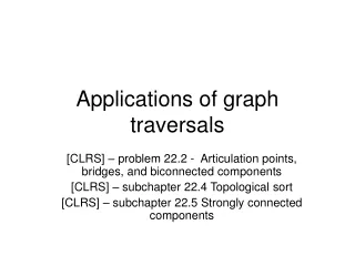
38. DAGs describe precedence • Examples: • prerequisites for a set of courses • dependencies between programs • job schedules • Edge from a to b indicates a should come before b

39. DAGs Describing Precedence Batman images are from the book “Introduction to bioinformatics algorithms”

40. No edges point backwards

41. Topological Sorting of DAGs • Topological sort: listing of nodes such that if (a,b) is an edge, a appears before b in the list • Is a topological sort unique?

43. Topological sort example • Give all possible DFS time stamps: S U V

44. Topological sort example S S S 1,6 1,6 5,6 U U U 2,5 1,4 4,5 V V V 3,4 2,3 2,3 S S 3,6 5,6 U U 3,4 4,5 V V 1,2 1,2 For all these time orderings Fv < FU < FS

45. Topological Sort • A DAG (directed acyclic graph) can be topologically sorted, ie linearly ordered so that predecessors come before successors, using depth first search. • Cormen et. al. show that for any edge (u,v) in a DAG finishing timestamp f(v) < f(u). Check previous example. • So when v is finished, put it in front of the list.

46. Conclusion: Topological sort • Run DFS • As each node is finished insert it in front of a linked list of nodes

47. Strongly Connected Components • A directed graph can be partitioned in strongly connected components: maximal sub-graphs C where for every u and v in C there is a path from u to v and there is a path from v to u.  • In a strongly connected component (SCC) all nodes can reach each other.

48. B A S C T SCCs ?

49. B A S C T SCCs: {A} {B} {C} {S,T}

50. SCC of GT • Given graph G=(V,E) define graph GT=(V,ET), where ET is the set of reversed edges of E. • G and GT have exactly the same SCCs! The path that went from x to y now goes from y to x, and vice versa.