High-Frequency MOSFET Analysis and Miller's Theorem Application

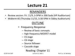
1. Lecture 21 REMINDERS • Review session: Fri. 11/9, 3-5PM in 306 Soda (HP Auditorium) • Midterm #2 (Thursday 11/15, 3:30-5PM in Sibley Auditorium) OUTLINE • Frequency Response • Review of basic concepts • high-frequency MOSFET model • CS stage • CG stage • Source follower • Cascode stage Reading: Chapter 11

2. Av Roll-Off due to CL • The impedance of CL decreases at high frequencies, so that it shunts some of the output current to ground. • In general, if node j in the signal path has a small-signal resistance of Rjto ground and a capacitance Cj to ground, then it contributes a pole at frequency (RjCj)-1

3. Pole Identification Example 1

4. Pole Identification Example 2

5. Dealing with a Floating Capacitance • Recall that a pole is computed by finding the resistance and capacitance between a node and (AC) GROUND. • It is not straightforward to compute the pole due to CF in the circuit below, because neither of its terminals is grounded.

6. Miller’s Theorem • If Av is the voltage gain from node 1 to 2, then a floating impedance ZF can be converted to two grounded impedances Z1 and Z2:

7. Miller Multiplication • Applying Miller’s theorem, we can convert a floating capacitance between the input and output nodes of an amplifier into two grounded capacitances. • The capacitance at the input node is larger than the original floating capacitance.

8. Application of Miller’s Theorem

9. MOSFET Intrinsic Capacitances The MOSFET has intrinsic capacitances which affect its performance at high frequencies: • gate oxide capacitance between the gate and channel, • overlap and fringing capacitances between the gate and the source/drain regions, and • source-bulk & drain-bulk junction capacitances (CSB & CDB).

10. High-Frequency MOSFET Model • The gate oxide capacitance can be decomposed into a capacitance between the gate and the source (C1) and a capacitance between the gate and the drain (C2). • In saturation, C1 (2/3)×Cgate, and C2  0. • C1 in parallel with the source overlap/fringing capacitance  CGS • C2 in parallel with the drain overlap/fringing capacitance  CGD

11. Example …with MOSFET capacitances explicitly shown Simplified circuit for high-frequency analysis CS stage

12. Transit Frequency • The “transit” or “cut-off” frequency, fT, is a measure of the intrinsic speed of a transistor, and is defined as the frequency where the current gain falls to 1. Conceptual set-up to measure fT

13. Small-Signal Model for CS Stage

14. … Applying Miller’s Theorem Note that wp,out > wp,in

15. Direct Analysis of CS Stage • Direct analysis yields slightly different pole locations and an extra zero:

16. I/O Impedances of CS Stage

17. CG Stage: Pole Frequencies CG stage with MOSFET capacitances shown

18. AC Analysis of Source Follower • The transfer function of a source follower can be obtained by direct AC analysis, similarly as for the emitter follower (ref. Lecture 14, Slide 6)

19. Example

20. Source Follower: Input Capacitance • Recall that the voltage gain of a source follower is Follower stage with MOSFET capacitances shown • CXY can be decomposed into CX and CY at the input and output nodes, respectively:

21. Example

22. Source Follower: Output Impedance • The output impedance of a source follower can be obtained by direct AC analysis, similarly as for the emitter follower (ref. Lecture 14, Slide 9)

23. Source Follower as Active Inductor CASE 1: RG < 1/gm CASE 2: RG > 1/gm • A follower is typically used to lower the driving impedance, i.e. RG is large compared to 1/gm,so that the “active inductor” characteristic on the right is usually observed.

24. Example

25. MOS Cascode Stage • For a cascode stage, Miller multiplication is smaller than in the CS stage.

26. Cascode Stage: Pole Frequencies Cascode stage with MOSFET capacitances shown (Miller approximation applied)

27. Cascode Stage: I/O Impedances