Understanding Active Galactic Nuclei Through Fe Lines in X-ray Astronomy
Learn about Fe fluorescence line at 6.4 keV, AGN accretion disks, General Relativity effects near black holes, and ionization theories. Explore spacecraft attitude, boresight alignment, and X-ray instrumentation calibration. Discover insights on Fe lines in AGN and Kerr metric.

Understanding Active Galactic Nuclei Through Fe Lines in X-ray Astronomy
E N D
Presentation Transcript
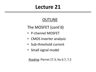
Lecture 21 • 6.4 keV Fe line and the Kerr metric • Satellite observatories • Attitude and boresight • X-ray instrumentation and calibration (mostly XMM). • (XMM users’ guide: • http://xmm.esac.esa.int/external/xmm_user_ support/documentation/uhb/index.html)
Fe lines in AGN – what this can tell us about GR • Fe: iron of course. There is a fluorescence line at 6.4 keV (in the rest frame). • AGN: Active Galactic Nucleus. • No-one has seen one close up – but almost certainly, these are accretion disks about a large black hole. • GR: here this doesn’t mean gamma ray, but General Relativity. • We expect to see GR effects near a giant black hole, because the gravitational force is so extreme.
(Tentative) cross-section through an AGN: To us Flare Jet Continuum background from halo Fe fluor. Flare additional continuum Accretion disk BH Accretion disk halo hot Very Innermost stable orbits – about 6rg for non-spinning BH; closer in for spinning BH. Jet
Fluorescence from a ‘cool reflector’. From A Fabian et al, PASP 112, 1145 (2000)
How ionization modifies this From A Fabian et al, PASP 112, 1145 (2000)
A Doppler-broadened spectral line – predictions of various theories: An accretion disk seen from above: Slow – small DS Profiles just for the two dashed annuli. Fast – large DS Fainter outside for whole disk Brighter inside From A Fabian et al, PASP 112, 1145 (2000)
Theory - spinning vs non-spinning BH Spinning (so-called Kerr-metric BH) Non-spinning (so-called Schwartzschild BH) From A Fabian et al, PASP 112, 1145 (2000)
Time-varying behaviour in MGC -6-30-15.This is a Seyfert I galaxy. From Tanaka et al (1995). 1997: time-averaged. 1994: time-averaged. 1994: in a deep minimum. 1997: at flare peak. From A Fabian et al, PASP 112, 1145 (2000)
Attitude • The orientation of the spacecraft in the sky is called its attitude. • It isn’t just the direction it points to, attitude specifies the roll angle as well. • One way to define this is via a pointing vector and a parallactic angle. • However, as with any trigonometric system, this has problems at poles. • Better is to define a Cartesian coordinate frame of 3 orthogonal vectors. • Each vector defined by direction cosines in the sky frame. • Attitude is then an attitude matrixA. • This is isotropic (no trouble at poles). • Easy to convert between different reference frames. • Whatever you do, avoid messing about with Euler angles. Ugh.
Sky frame or basis. z at dec=90° Unless you have good reason not to, always construct a Cartesian basis according to the Right-Hand Rule: xy screws toward z; yz screws toward x; zx screws toward y. y at RA=6 hr x at RA=0 “Direction cosines” really just means Cartesian coordinates.
RA/dec Cartesian (ie, direction cosines). z at dec=90° y at RA=6 hr x at RA=0 To invert this:
Spacecraft basis (green vectors). zsky Attitude matrix: xs/c ysky xsky ys/c zs/c
Conversion from sky to spacecraft basis: zsky Attitude matrix: xs/c ysky xsky ys/c zs/c Inverting it:
Boresights • Ideally, each instrument on a satellite would be perfectly aligned with the spacecraft coordinate axes. • In real life, there is always some misalignment. This is called the boresight of the instrument (I think it is an old artillery term). • Define a set of Cartesian axes for each instrument. • Components of these axes in the spacecraft reference system (basis) form the boresight matrix Bfor that instrument.
Boresights • With these matrices, conversion between coordinate systems is easy. Suppose we have an x-ray detection which has a position vector v|inst in the instrument frame. If we want to find where in the sky that x-ray came from, we first have to express this vector in the sky frame Cartesian system (new vector = v|sky). This is simple. Since we have: • then
Attitude and boresights • NOTE that attitude varies with time as the spacecraft slews from target to target – but there is ALSO attitude jitter within an observation. • XMM has a star tracker to measure the attitude. • Attitude samples are available at 10 second intervals. • So to build up a sky picture from x-ray positions in the instrument frame, one has to change to a new attitude matrix whenever the deviation grows too large. • Boresights can also change with time, due to flexion of the structure, but this is slow. • Calibration teams measure them from time to time.
Other coordinate systems: • The fundamental spatial coord system is the chip coordinate system – in CCD pixels. • Note that for time and energy as well as in the spatial coordinates, coordinate values are ultimately pixellized or discrete. • This defines the uncertainty with which they are known (to ±half the pixel width). • Rebinning can give rise to Moiré effects (somewhat similar to aliasing in the Fourier world). • ‘Dithering’ can avoid this.
X-ray Observatories • You need to be in space, because the atmosphere efficiently absorbs x-rays. • Most of the currently interesting results are coming from: • Chandra (good images, so-so spectra) • XMM-Newton (so-so images, good spectra) • SWIFT (looks mostly at GRB afterglows) although there are several more. • How do you make an image from x-rays? Don’t they go through everything? So how can you make a reflector?
X-ray Observatories - mirrors • Wolter grazing-incidence mirrors: • reflectivity of any EM radiation gets higher for a low angle of incidence. Double reflection Can nest many shells of differing diameter. Paraboloid Hyperboloid Behaves like a thin lens set here.
X-ray Observatories - detectors • Charge Coupled Devices (CCDs) are used, just as for optical. The workings are slightly different though. e- e- e- e- e- e- e- e- e- e- e- e- e- e- e- e- e- e- e- e- e- ...then read out. At optical wavelengths: At x-ray wavelengths: e- e- e- e- e- e- e- e- e- e- e- e- e- ...then read out. Time
X-ray Observatories - detectors • Basic substance of the CCD is silicon – but ‘doped’ with impurities which alter its electronic structure. • There are several sorts, eg: • Metal Oxide Semiconductor (MOS) • pn • The CCD surface is divided into an array of pixels. • A photon striking the material ejects some electrons which sit around waiting to be harvested. • The number of ejected electrons is proportional to the energy of the photon.
X-ray Observatories - detectors • CCD operation is in frame cycles. Long accumulation time Short readout time
X-ray Observatories - detectors • CCDs have to be read out sequentially (slow). Columns Rows Digitizer (ADC) Out Readout row
X-ray Observatories - detectors • The readout operation consists of the following steps: • For each CCD row, starting with that nearest the readout row, move the charges into the next lowest row. • In the readout row, starting at the pixel nearest the output, shift the charges into the next lowest pixel. • Convert the analog charge quantity (it is an integer number of electrons, but such a large integer that we can ignore quantum ‘graininess’) to a digital number. • This is done in an Analog to Digital Converter (ADC). • Send that number to the outside world.
X-ray Observatories - detectors • For x-ray detection, we want to arrange the frame duration so that we expect no more than 1 x-ray per pixel per frame. • Why? Because if we can be pretty sure that all the charge per pixel per frame comes from a single x-ray, we can determine the energy of the x-ray. x-ray spectroscopy. • XMM example: • Spatial resolution is ~1 arcsec (fractional ~10-3). • Spectral resolution is ~100 eV (fractional ~10-2). • Time resolution is ~1 second (fractional ~10-5).