Charles University

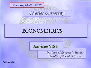
Tuesday, 14.00 – 15.20 Charles University Charles University Econometrics Econometrics Jan Ámos Víšek Jan Ámos Víšek FSV UK Institute of Economic Studies Faculty of Social Sciences Institute of Economic Studies Faculty of Social Sciences STAKAN III Sixth Lecture

Schedule of today talk First pattern of output from statistical package. Misinterpretations of results and how to avoid it. Is the estimated model acceptable or not? (Verifying the assumptions for OLS to be BLUE.) (Consistency and normality will be next time.)

Types of statistical libraries (packages) Menu-oriented  all required evaluations are made “by clicking the mouse” STATISTICA , E-views Key-oriented  required evaluations are performed as sequence of orders written by means of key-words TSP, SAS , S-PLUS, R Combined

A first pattern of statistical package output Regression Summary for Dependent Variable: CCAS R= .92364067 R²= .85311209 Adjusted R²= .82961003 F(4,25)=36.299 p<.00000 Std.Error of estimate: 28.671 Estimates of coefficients in model for transformed data. Estimates of coefficients in model for original data. (For further discussion Remember the Fifth Lecture of columns of the table see the next slide.)

A first pattern of statistical package output Regression Summary for Dependent Variable: CCAS R= .92364067 R²= .85311209 Adjusted R²= .82961003 F(4,25)=36.299 p<.00000 Std.Error of estimate: 28.671 Clearly insignificant, but ..... Slightly insignificant Remember again Evidently insignificant Surely significant the Fifth Lecture

One of frequently appearing misinterpretation of model: Assume that the result of regression analysis was Time Total =-3.62 + 1.27 * Weight - 0.53 * Puls - 0.51 * Strength + 3.90 * Time per ¼-mile. Then we can frequently meet with a conclusion of type “As the estimate of regression coefficient for Weight is positive, the Weight has positiveimpacton Time Total .” or (even) “Although the coefficient of determination is small, the po- larity of the estimated coefficients corresponds to our ideas.”. The first assertion can be true, under some circumstances, but generally we cannot claim anything like that. The second assertion can have, under some circumstances, a sense but generally is false. Why?

Let us consider following, a bit academic, example: The regression model has random explanatory variables and the shape . (1) Moreover, but we are not aware of this relation between and and we take into account only (1). If we conclude that has positive impact on , it is surelyfalse conclusion. What to do? Remember “Ceteris paribus” - - unfortunately, it’s an academic illusion !!

The relation (2) or a similar one cannot be “discovered” by correlation analysis. The correlation indicates only linear relations among r.v.’s. Sorry! But if we take into account correlation matrix of ( with , of course ) we have a chance, again due to Weierstrass theorem, to find some latent relations between (keep in mind that not among) the explanatory variables. Denote this matrix by .

Of course, the best is to try to regress one explanatory variable on various combinations of others, their functions, powers etc. Clearly, it is tiresome, time-consuming job, full of routine,etc. In STATISTICA Running regression , we obtain as an indication of collinearity the table “Redundancy” containing all coefficients of determination of models which regresses one column of on all other columns. We shall speak about collinearity later on.

Sometimes, a grain of intuition is better than hours of routine. I would like to have a drop of good luck, or a barrel of intelligence !! Menandros, 342 – 293 B.C. After all, analysis of data is, at least partially, an art. (Or the art ?!) Let us recall that we have already showed another possible misinterpretation - namely how misleading can be to infer on the impact of given explanatory variable on the response from the magnitude of estimated coefficient. See the Fifth Lecture, the fourth slide

We already know that we should ...... To estimate the model which includes only significant explanatory variables. To check that the coefficient of determination is acceptably large. To find out the mutual relations of explanatory variables. Can we then accept model and interpret it? I am sorry, not yet !! What should we do more? A hint: The answer can be deduced from what was already given !!! The answer is as simple as follows: We should check the assumptions under which the OLS are optimal estimator !!

Let us recall - Theorem Assumptions Let be a sequence of r.v’s, . Assertions Then is the best linear unbiased estimator . Assumptions If moreover , and ‘s are independent, Assertions is consistent. Assumptions If further , regular matrix, Assertions then where . Prior to looking for a way how to verify the assumptions, let us also recall the picture, graphically showing ......

Recall that and Y .

Testing validity of the assumptions Sometimes we can meet with idea that showing that is small, the assumption will be verified. However, as we have seen on previous slide, it holds always. Moreover, the assumption is in fact accommodated by the ( linear ) regression model. Notice that in the case when , we can consider model with . In other words, the assumption cannot be and even need not be verified.

Testing validity of the assumptions (homoscedasticity) The most of test of the homoscedasticity are based on testing an idea about the model of heteroscedasticity. We are going to show one of them but there are plenty of such tests – rarely implemented. Another test will not be from this class, it is based on surprisingly simple idea and it is frequently used.

Breusch-Pagan test (1979) Assumptions Assume that where h is a (smooth) function and . Denoting , we observe that if null hypothesis is valid, then are not significant ( we will learn later how to test simultaneously whether several coefficients are not significant). Assertions The locally most powerful test can be based on the statistic powerful against skew d.f. of ’s with , .

White’s test (1980) Prior to the explanation notice that Technicalities and recall that . Moreover, if random variables and are independent, . The idea of test is given by .

White’s test (1980) Continued So, the idea of test is to compare two matrices and . Test is in fact carried as follows (Halbert White, 1980) Assumptions Put and regress on , i.e. consider the regression model . Assertions Then for its coefficient of determination we have L ( ) .

White’s test (1980) Continued Of course, libraries (e.g. TSP, E-Views) give the corresponding p-value that r.v. is larger than value of resulting from the regression given on the previous slide. Again technicalities Let us recall that and hence and hence can be estimated by . However, if , we obtain Remember this matrix! .

White’s test (1980) – consequence for looking for a model Continued Halbert White showed that can be consistently estimated by . So if the hypothesis about homoscedasticity is rejected, we should (or better, has to) studentize the coordinates of estimate . by the square root of diagonal elements of matrix We shall recall what it is on the next slide !

Recalling studentization Lemma Assumptions Let be iid. r.v’s, . Moreover, let and be regular. Assertions Put Then . Assumptions Put where , is called then studentization. , where This transformation . is called studentization. By it we rid of which is unknown. Then , i.e. is distributed as Student with degrees of freedom. Assertions

White’s test (1980) – consequence for looking for a model Continued Lemma Assumptions So, similarly as in previous, we put where however now . Assertions Then again . What can happen if heteroscedasticity is recognized but ignored, demonstrates the example on the next slide.

Model of export from the Czech republic into EU 29 industries: Agriculture and hunting , Forestry and logging, Fishing, Mining of coal and lignite,Other mining, Manufacture of food products and beverages, Man.of tobacco products, Man. of textiles, Man. of textile products for the household, Man. of footwear, Man. of wood and of products of wood , Man. of pulp, paper and paper products, Publishing, printing and reproduction,Man. of coke, refined petroleum products and nuclear fuel, Man. of chemicals and phar- maceuticals, Man. of rubber and plastic products, Man. of bricks, tiles, constr. products and glass, Man. of basic metals, Man. of struc- tural metal products,Man. of machinery , Man. of office machinery, Manufacture of electrical machinery and apparatus, Radio, television and communication equipment, Medical, precision and optical instruments, Motor vehicles, Transport equipment , Furniture, Recycling, Electricity, gas, steam and hot water supply 1993 - 2001

Response variable: Export from the Czech republicinto EU Explanatory variables : PE/kg, PI/kg, Tariffs from EU on X, Tariffs CZ on M, Prize deflator (base 94), FDI stock , K/L, EMPloyment, Value Added, GDPeu (total), GDPcz (total), REER, Wages, Annual cost, Total expenditure, Debts Some preliminary analysis ( we shall speak about it later - - may be in summer term ) indicated that also past values of explanatory variables should be used.

Example of model ignoring heteroscedasticity Notice that all explanatory variables are significant!

Other characteristics of model

This is the signifikance of coefficients when White estimate of covariance matrix was employed Notice that nearly all explanatory variables are non-significant!

Employing White estimateof covariance matrix of the estimates of regression coefficients Resulting model is considerably simpler !!!

Other characteristics of model Notice that the heteroscedasticity is not removed, only (?) the significance was judged on modified values of studentized estimates of regression coefficients !!

Warning !!! Attempts of removing heteroscedasticity by a transformation of data is typically the reliable way to hell !!! The only exception may be when the shape of heteroscedasticity is know with high degree of reliability. An example: Data are aggregated values of some economic, demographic, sociologic,educational, etc. characteristics over districts of a country. Then the variance of these givens are inversely proportional to the number of inhabitants, economic subjects, etc. Then there is a grain of hope that .........

Analyzing homoscedasticity by graphic tools The idea: If , then should not depend on i . So plotting against i , we should not obtain any regular or periodical shape of graph. Such graph is called index plot . A “handicap” of the idea is that the shape of graph depends on the order of observations in analyzed data. Hence one can easily reorder the data so that we obtain a regular shape of graph. A remedy is simple !

Analysing homoscedasticity by graphic tools The refined idea: If then should not depend on and/or. So plotting e.g. against , we should not obtain any regular shape ...... . (An example is on the next slide.) Looking for heteroscedasticity by circumstances Assume the consumption of households. Those with large income do not consume all but save some money and buy, from time to time, TV-set, fridge, car, etc. . It means that their consumption is sometimes smaller sometimes larger while the consumption of poorer households is nearly the same all the time. Hence the consumption will not be (usually) homoscedatic.

Squared residuals plotted against predicted values of response. The result indicates that a suspicion on a slight heteroscedasticity can arise.

Let us recall once again - Theorem Assumptions Let be a sequence of r.v’s, . Assertions Then is the best linear unbiased estimator . Assumptions If moreover , and ‘s are independent, Assertions is consistent. Assumptions If further , regular matrix, Assertions then where . There are still some assumptions to be verified. We’ll discuss them on the next lecture.

What is to be learnt from this lecture for exam ? Linearity of estimator and of model – what advantages and restrictions do they represent ? How to test basic assumptions: - , - homoscedasticity : White test versus tests based on model of heteroscedasticity, i.e. two approaches based on different ideas ? - graphic tests? What means : “The estimator is the best in the class of ….” OLS is the best unbiased estimator - the condition(s) for it. All what you need is on http://samba.fsv.cuni.cz/~visek/

Charles University