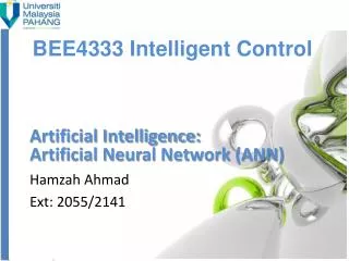
BEE4333 Intelligent Control

1. Artificial Intelligence: Artificial Neural Network (ANN) BEE4333 Intelligent Control Hamzah Ahmad Ext: 6024/6130

2. Todays Lesson • 4.1 Basic Concept • 4.2 ANN Applications • LO1 : Able to understand the concept of Artificial Neural Network and its applications

3. Basic Concept • ANN born from the demand of machine learning; computer learns from experience, examples and analogy. • Simple concept : computer attempts to model the human brain. • Also known as parallel distributed processors. • Why we need an intelligent processor or computer to replace current technology? • To decide intelligently and interact accordingly.

4. Human Brain; biological NN Synapses; connection between neutrons Axon; sends information SOMA SOMA Dendrites; Received information NEURON Learning from experience! Plasticity : Neurons heading to right answer are strengthen and for the wrong answer is weakened.

5. Learning OUTPUT SIGNALS INPUT SIGNALS INPUT LAYER MIDDLE LAYER OUTPUT LAYER ANN Architecture

6. Learning • Synapses has their own weight to express the importance of input. • ANN learns through iterated adjustment from synapses weight. • Weight is adjusted to cope with the output environment regarding about its network input/output behavior. • Each neutron computes its activation level based on the I/O numerical weights. • The output of a neuron might be the final solution or the input to other networks.

7. How to design ANN? • Decide how many neurons to be used. • How the connections between neurons are constructed? How many layers needed? • Which learning algorithm to be apply? • Train the ANN by initialize the weight and update the weights from training sets.

8. ANN characteristics Advantages: • A neural network can perform tasks that a linear program can not. • When an element of the neural network fails, it can continue without any problem by their parallel nature. • A neural network learns and does not need to be reprogrammed. • It can be implemented in any application. • It can be implemented without any problem. Disadvantages: • The neural network needs training to operate. • The architecture of a neural network is different from the architecture of microprocessors therefore needs to be emulated. • Requires high processing time for large neural networks.

9. Todays Lesson • 4.3 ANN Model • 4.4 ANN Learning • 4.5 Simple ANN • LO1 : Able to understand basic concept of biases, thresholds and linear separability • LO2 : Able to analyze simple ANN (Perceptrons)

10. Examples of ANN

11. Categorization Feedforward • All signals flow in one direction only, i.e. from lower • layers (input) to upper layers (output) Feedback • Signals from neurons in upper layers are fed back • to either its own or to neurons in lower layers. Cellular • Connected in a cellular manner.

12. Exercise • Construct 4 artificial neurons • 2 neurons on the input and 2 neurons on the output • Each arrow has its own weight. • Those weight is multiplied to each value going through each arrow - what this process define? • If there is only ONE (1) input and a weight, so the output will be the multiplication of both. For more than ONE (1) input and weights, then the neuron will sum up the values. • Consider the weight is ONE (1) for each arrow and set the input to be (0,0), (0,1), (1,1), (1,-1), (-1,1). • What happens? • Change the weight randomly and differently between -0.5 to 0.5 to each arrows. What happens? • Try changing the weight again other than above weights. • Observed what happen.

13. ANN Learning • In all of the neural paradigms, the application of an ANN involves two phases: • (1) Learning phase (pengajaran) • (2) Recall phase (penggunaan) • In the learning phase (usually offline) the ANN is trained until it has learned its tasks (through the adaptation of its weights) • The recall phase is used to solve the task.

14. ANN Learning • An ANN solves a task when its weights are adapted through a learning phase. • All neural networks have to be trained before they can be used. • They are given training patterns and their weights are adjusted iteratively until an error function is minimized. • Once the ANN has been trained no more training is needed. • Two types of learning prevailed in ANNs: • Supervised learning:- learning with teacher signals or targets • Unsupervised learning:- learning without the use of teacher signals

15. Supervised Learning • In supervised learning the training patterns are provided to the ANN together with a teaching signal or target. • The difference between the ANN output and the target is the error signal. • Initially the output of the ANN gives a large error during the learning phase. • The error is then minimized through continuous adaptation of the weights to solve the problem through a learning algorithm. • In the end when the error becomes very small, the ANN is assumed to have learned the task and training is stopped. • It can then be used to solve the task in the recall phase.

16. Supervised Learning Matching the I/O pattern

17. Unsupervised Learning • In unsupervised learning, the ANN is trained without teaching signals or targets. • It is only supplied with examples of the input patterns that it will solve eventually. • The ANN usually has an auxilliary cost function which needs to be minimized like an energy function, distance, etc. • Usually a neuron is designated as a “winner” from similarities in the input patterns through competition. • The weights of the ANN are modified where a cost function is minimized. • At the end of the learning phase, the weights would have been adapted in such a manner such that similar patterns are clustered into a particular node.

18. ANN paradigm • There are a number of ANN paradigms developed over the past few decades. • These ANN paradigms are mainly distinguished through their different learning algorithms rather than their models. • Some ANN paradigms are named after their proposer such as Hopfield, Kohonen, etc. • Most ANNs are named after their learning algorithm such as Backpropagation, Competitive learning, Counter propagation, ART, etc. and some are named after their model such as BAM, • Basically a particular ANN can be divided into either a feedforwardor a feedback model and into either a supervised or unsupervised learning mode.

19. ANN Classifications

20. ANN Performance • The performance of an ANN is described by the figure of merit, which expresses the number of recalled patterns when input patterns are applied, that could be complete, partially complete, or even noisy. • A 100% performance in recalled patterns means that for every trained input stimulus signal, the ANN always produces the desired output pattern.

21. ANN Performance

22. Basis of ANN computing idea • Neuron computes the input signals and compares the result with a threshold value, θ. • If the input is less than θ, then the neuron output is -1, otherwise+1. • Hence, the following activation function(sign function) is used, where X is the net weighted input to neuron, xiis the iinput value, wiis the weight of input i . n is the number of neuron input and Y is the neuron output.

23. Other types of activation function Step function Sigmoid function Y Y Y Y +1 +1 +1 +1 0 0 0 0 X X X X Sign function Linear function -1 -1 -1 -1 X

24. Simple ANN: A Perceptron • Perceptron is used to classify input in two classes; e.g class A1 or A2. • A linear separable function is used to divide the n-dimensional space as follows; • Say, 2 inputs, then we have a characteristics as shown on left figure. θ is used to shift the bound. • Three dimensional states is also possible to be view. x2 1 0 x1 2

25. Simple Perceptron Must be boolean! Inputs x1 Linear Combiner Hard limiter w1 Output/bias ∑ x2 w2 θ Threshold

26. Different training pattern based on weights defined Decision boundary • Note that p1 and p2 are incorrectly being determined • p1 target is t=1 and p2 target is t=-1

27. Learning: Classification • Learning is done by adjusting the actual output Y to meet the desired output Yd. • Usually, the initial weight is adjust between -0.5 to 0.5. At iteration k of the training example, we have the error e as • If the error is positive, the weight must be decrease and otherwise must be increase. • Perceptron learning rule also can be obtained where α is the learning rate and 0<α<1.

28. Training algorithm • Step 1: Initialization • Set initial weight wi between [-0.5,0.5]and θ. • Step 2: Activation • Perceptron activation at iteration 1 for each input and a specific Yd. e.g for a step activation function we have • Step 3: Weight training • Perceptron weight is updated by where =αX xi(p) Xe(p) • Step 4: Iteration • Next iteration at time k+1 and go to step 2 again.

29. Example • Consider truth table of AND operation • How ANN of a single perceptron can be trained? • Consider a step activation function in this example. Threshold, θ = 0.2 Learning rate, α = 0.1 Use initial weight as 0.3 for x1and -0.1 for x2

30. where =αxxi(p) x e(p) The epoch continues until the weights are converging to a steady state values.

31. Now consider this problem • Design a mobile robot that avoid collisions using ANN. • There are three inputs; right wheel velocity, left wheel velocity and relative distance between robot and obstacle. • The output will be the mobile robot heading angle. • Write only two epoch for this problem.

32. Today Lessons • 4.3 ANN Model • 4.4 ANN Learning • 4.5 Simple ANN • LO1 : Able to understand basic concept of biases, thresholds and linear separability • LO2 : Able to analyze simple ANN (Perceptrons)

33. Today Lessons • 4.6 Multilayer Neural Networks & Backpropagation Algorithm • LO1 : Able to understand basic concept of biases, thresholds and linear separability

34. Sigmoid function characteristics • The sigmoid activation function with different values c. • When c is large, the sigmoid becomes like a threshold function and when is c small, the sigmoid becomes more like a straight line (linear). • When c is large learning is much faster but a lot of information is lost, however when c is small, learning is very slow but information is retained. • Because this function is differentiable, it enables the B.P. algorithm to adapt the lower layers of weights in a multilayer neural network. • Because this function is differentiable, it enables the B.P. algorithm to adapt the lower layers of weights in a multilayer neural network.

35. Multilayer neural networks • Multilayer NN-feedforward neural network with one or more hidden layer. • Model consists of input layer, middle or hidden layer and an output layer. • Why hidden layer is important? • Input layer only receives input signal • Output layer only display the output patterns. • Hidden layer process the input signals; weight represents feature of inputs.

36. Multilayer NN model Inputs Output x1 x2 x3 2nd hidden layer 1st hidden layer

37. Multilayer Neural Network learning • Multilayer NN learns through a learning algorithm; the popular one is BACK-PROPAGATION. • The computations are similar to a simple perceptron. • Back-propagation has two phases; • Input layer demonstrates the training input pattern and then propagates from layer to layer to output. • The calculation for error will notify the system to modified the weights appropriately.

38. Back-propagation • Each neurons must be connected to each other. • Calculations • Same as a simple perceptron case. • Typically, sigmoid function is used in Multilayer NN.

39. Back-propagation: Learning mode • Before the BP can be used, it requires target patterns or signals as it a supervised learning algorithm. • Training patterns are obtained from the samples of the types of inputs to be given to the multilayer neural network and their answers are identified by the researcher. • Examples of training patterns are samples of handwritten characters, process data, etc. following the tasks to be solved. • The configuration for training a neural network using the BP algorithm is shown in the figure below in which the training is done offline. • The objective is to minimize the error between the target and actual output and to find ∆w.

40. BP: Learning mode • The error is calculated at every iteration and is backpropagated through the layers of the ANN to adapt the weights. • The weights are adapted such that the error is minimized. • Once the error has reached a justified minimum value, the training is stopped, and the neural network is reconfigured in the recall mode to solve the task.

41. Error gradient

42. Let’s look for a specific case wij yi xi wjk m n l inputs i j output k Input signals Error signals

43. Understand more, learns more • Error propagation starts from output layer back to hidden layer. • How to calculate error signals at layer k? • How about calculation to update the weights at layer k? • Weight correction; • or • In sigmoid function, where

44. Weight correction in hidden layer • We use the same technique to find the weight in hidden layer.

45. Steps for calculations • Step 1 : Initialization • Set weights and threshold randomly within a small range • Step 2 : Activation • Use sigmoid activation function at hidden layer and output layer • Hidden layer; • Output layer;

46. Step for calculations • Step 3 : Weight training • Calculating error gradient in output layer where Update ; • Calculating error gradient in hidden layer Update ; • Step 4 : Iteration • Back to step 2 and repeat process until selected error criterion is satisfied.

47. When does the training process stop? • Training process stop until the sum of squared error for the output yis less than a prescribed value; 0.001. • Sum of squared error : performance indicator of the system. • The smaller, the better the system performance.

48. More about back-propagation • Different initial weights and threshold may have different solutions, but finally the system has almost similar solutions. • The decisions boundaries can be view if we use the sign activation function. • Drawbacks of back-propagation • Not suitable for biological neurons; to adjust the neurons weight. • Computational expensive • Slower training

49. Consider other technique Sigmoid function; f(x) = (1+e-x)-1 f(x) = x The error signals are as follows. δk = Lk (1- Lk )( tk - Lk ) δj = Lj(1- Lj ) ∑kδkwkj Adaptions of weights are defined as below. ∆wkj( t + 1) = η δkLj + α∆wkj( t ) ∆wji( t + 1) = η δj Li + α∆wji( t )

50. XOR PROBLEM