Architectural-level Design Exploration for Power Aware System
390 likes | 565 Vues
Architectural-level Design Exploration for Power Aware System. Dexin Li October 2000. Background . Component-level low power design cannot meet system-level design goals System needs not only low power designs, but also power aware features. Motivation.

Architectural-level Design Exploration for Power Aware System
E N D
Presentation Transcript
Architectural-level Design Exploration for Power Aware System Dexin Li October 2000
Background • Component-level low power design cannot meet system-level design goals • System needs not only low power designs, but also power aware features
Motivation • System architecture is important for power aware system designs • Our micro-rover example shows bus/bus interface consume 25.65% of total system power • By adopting a variety of low-power design techniques and low power components, architectural optimization becomes more important.
Application Example • Microrover - Robot exploring Mars • Solar power: 15W @noon • Electronics system: • Processor, microcontroller • Camera • radio frequency modem • Non-volatile memory/hard drive • Scientific equipment: APXS & ASI/MET • Bus drivers • System tasks: • Steering and driving • Capture pictures and send compressed data • Perform scientific experiments, store data on media, and send data
Previous Work • A lot of lower power design techniques • Voltage scaling, frequency scaling, clock gating • Bus encoding, bus segmentation • Algorithm transformation, imprecise arithmetic • Other Power Aware methodology • PACT: on demand control of power consumption and performance • µAMPS: adaptive energy-aware distributed microsensors
IMPACCT methodology • A framework to enable power aware design • Behavioral level optimization • Scheduling, partitioning, migration • Architectural level design exploration • Constraint-driven design space exploration • Meet power and performance constraints • Different view of system behavior, thus different solution • Static, know system behaviors prior to architecture exploration • Mixed, hybrid, prepare solutions for a few scenarios, pick up one at run time • Dynamic, determine the system behaviors and explore design space both at run time,
Assumptions for the problem • Use COTS component to construct system • Communication • Un-directional • Components’ stand-alone time is absorbed into communication time (at coarse granularity) • Static view of the system behavior
Problem statement • Design a tool(algorithm) that comes up with an architectural topology and power management scheme that satisfy system-level power, workload and schedule constraints. • Input: • Component property • Workload graph • Behavioral schedule • System constraints • Output: • A feasible architecture • power management scheme
Component property • Component name • Power modes • Communication bandwidth • Mapping table • Performance / power • Clock frequency / power • Supply voltage / power • Bus interface • Maximum fanout • Root node eligibility(Can be root node or not)
mc1 sc1 cam 40 40 20 cpu1 2 20 180 hd cpu2 mc1 5 30 sc1 rf Workload graph • A representation of communication • Vertices: components • Edges: workload(data transfer rate) • Weight: required communication bandwidth
CPU1 MC1 MC2 CPU2 CAM RF HD SC1 SC2 10 20 30 40 50 min Behavioral schedule • Mission-level schedules • From behavioral scheduling or system specification • Communication-active and stand-alone-active • Granularity related • Here assumes they are same
System constraints • Power • Maximum power, constant • Maximum power, function of time • Power range, constant, function of time • Protocol • Topology: e.g. tree for 1394 bus • Communication bandwidth • 100, 200, 400Mbps for different 1394 bus components • Up to 80% of bandwidth for isochronous transfers
mc2 sc2 cpu1 mc1 hd cpu2 rf cam sc1 Output topology • A feasible topology meets all system constraints, if any
Output-PM scheme • Power management scheme • Working together with the output topology • Indicating results for each components, at each schedule interval • power mode • power consumption number • required bandwidth • Used as feedback to behavioral scheduling or software development
Problem Formulation • Tool elements: • Component library(CL) • Topology generator(TG) • Power management inspector(PMI) • Power calculator(PC) • With workload graph, TG first generates a graph from which different topology would be abstracted out; PMI sets working modes to each component, and check whether they are legal combinations. PC finds out power number for the entire system and see whether it meets power constraints. If yes, the problem is solved; if not, different working modes or different topology are tried, and check again.
Application FU BI Bus media BI FU Application LNK Full-on PHY sleep SUS Deep sleep Bus media Component Model • Component composition: • Functional unit (FU) • Bus interface (BI) • Power management model: • Layered power modes • Modes correspondence between FU and BI Suppose when FU is working, it has communication with other components.
application application TRS TRS LNK LNK PHY PHY Bus media sender receiver Bus Model • Sender and receiver • Service layers • Transfer property(modes, speed, bandwidth) • Configuration process
BI FU Data to be transferred from node A to C yes Application A B C LNK Full-on no PHY sleep SUS Deep sleep Node B can’t be put in SUS mode. Bus media Configuration Management I • Power modes constraints: • Intra-component constraints • Inter-component constraints
Data to be transferred from node A to C @ 400Mbps A B C A B C D Node B’s transfer speed should be 400Mbps, too Configuration Management II • Bandwidth constraints: Data transfer rates: A to D: 150Mbps B to D: 80Mbps Bandwidth for C: No less than 230Mbps For FireWire bus: 400Mbps
segmentation Low power design techniques I • Bus segmentation • Improve communication bandwidth • Power reduction by disable unused components or clusters • Enabling other low power design techniques
Low power design techniques II • Clock Scaling and Voltage scaling • Trade off between performance and power • Two or multiple levels of frequencies or voltages to select from • Extra hardware needed to implement the techniques
segmentation 400Mbps bus Using low power design techniques • Bus segmentation with clock scaling • With clustered bus, we can keep same bandwidth by lower the clock frequency for the communication 200Mbps cluster 100Mbps cluster Suspended cluster
Algorithm I • Creating Communication-Scheduling Table • Obtain combined information of both schedule and communication • Used for finding out constraint set for each component • Format: • CST : (tuple1, tuple2, ...) • Tuple1:(workload_path, interval, required_bandwidth) (('cpu2','mc1'),((20,30), 10)), (('cpu2','mc2'),((0,15), 20)), (('cpu1','cam'),((10,20), 20)), ...
Algorithm II • Building Constraint Set • Find legal modes • Working mode • Power mode • Bandwidth level • Constrained by • Topology • system schedule • communication Cam: ON: LNK Cam: WL: 120 Camera must be working at at least link-layer-on mode; Required bandwidth is 120Mbps, thus the bus driver should work at at least 200Mbps
Algorithm III • Enumerating topology • Complexity • pick up |Et| from |Eg|, |Et|, # of edges in the tree;|Eg|, # of edges in the graph 1. Start from workload graph G; 2. Add some redundant edges to G, we get G’; 3. Abstract valid topology T from G’ 4. Append T to topology library TL
Algorithm IV • Traversing Power management schemes • Grouping nodes into three classes: • Transferring (C1) • Passing (C2) • Idle(C3) • Traverse different combinations • Try bus segmentation and clock scaling techniques
Algorithm: top level 1.Reading in component property, workload graph, system schedule, and system constraints 2. Creating Communication-Scheduling Table 3. Building Constraint Set 4. Enumerating topology, building topology library TL 5. For Ti in TL : 6. For interval in schedule : 7. Traverse power management schemes PMSi; 8. Run power_calculator to find power number P for PMSi 9. If p satisfy power_constraint : 10. print “find a feasible solution”, Ti, PMSi 11. Stop 12. Print “can’t find a feasible solution”
MC1 SC1 SC2 30 30 20 CPU1 1 CPU2 20 160 MC2 10 20 NVM/HD RF CAM CPU1 MC1 MC2 CPU2 CAM RF HD SC1 SC2 10 20 30 40 50 min Example • FireWire 1394 bus architecture • Tree topology • Transfer speed 100, 200, 400Mbps • Application-Micro rover • 9 nodes • System schedule:walking, taking picture, walking and collect scientific data • Workload graph • power Constraints: • Constant value • Function of time • A range with max and min value or function
schedule workload Topology iterator topology Constraint set Power modes traversor Power calculator Component library Solution Experimental methodology • Constraint-driven design space exploration • Pre-given schedule from behavioral level to break the iteration loop • Proliferate the exploration space by adding some edges to original graph • Use both scheduling and communication information as knowledge, to build constraint set
CAM SC SC HD CPU MC 80 80 CPU HD MC 120 30 RF CAM 40 30 MAX_POWER constraint = 15.0W Actual MAX_POWER = 14.9W RF Experiments • Experiment 1:
SC CAM CPU HD MC CAM CPU RF MC MAX_POWER constraint = 14.0W Actual MAX_POWER = 13.94W SC RF HD 10 20 30 40 50 Experiments min
CPU2 HD CPU1 MC2 MC1 Power(W) RF CAM SC1 SC2 15 Power constraints 14 13 12 11 10 9 8 7 10 20 30 40 50 60 Experimental Results Time(min)
sc1 sc2 cam hd mc2 cpu1 mc1 rf cpu2
cam sc1 sc2 cpu2 hd mc2 cpu1 mc1 rf
Summary and future work • A tool to explore design space for power aware architecture • Meets different kinds of power constraints • Incorporate low power design techniques • Interaction with behavioral scheduling to refine solution • Future work: hybrid and dynamic exploration
Algorithm 1.Read in component property, communication graph, read system schedule, read system constraints; 2. Construct searching graph (SG); if |SG| > Max_SG then stop; 3. Construct schedule intervals Si; 4. Enumerate all the topologies from searching graph Ti SG 5. For each Ti do 6. { if Ti is topologically illegal then next Ti; 7. Build configuration constraints set(CCS)) for each component; 8. Initialize first schedule interval S1, all components in Full-on modes; 8. For each Si do 9. { if (Si != S1) copy power modes sets(PMSi) from previous interval; 10. While (PMSi not exhausted) 11. { If PMSi is legal then run power_calculator 12. { if system power satisfy power constraints then next Si; 13. Else next Ti; 14. } else 15. { find next PMSi; } 16. } 17. Next Ti ; 18. } print “find a solution:”; output Ti, PMS; stop 19. } 20. Go to step 2;